We are going to explore the entry requirements to visit a country across the globe. We will find out how easy or difficult to travel from one country to an other; which are most welcoming or reclusive nation according to what kind of travel documents they demand on entering their territories.
Preliminaries
Modules
The following modules and tools will be needed:
from collections import Counter
from itertools import chain, count, cycle, islice, product, repeat
import json

import ete3

from matplotlib import pyplot as plt
from matplotlib.colors import LogNorm, ListedColormap

import networkx as nx
import numpy as np
import pandas as pd
import seaborn as sns

from scipy.cluster.hierarchy import linkage
import scipy.stats as scs
import scipy.spatial.distance as scd

from sklearn.decomposition import PCA
from sklearn.metrics import fowlkes_mallows_score, silhouette_score
from sklearn.preprocessing import normalize
Utility functions
Firstly, a handful of helper functions are defined:
def load_dict_from_json(path_to_file):
    """
    Loads a dictionary from a json file
    Parameters:
        path_to_file (str) : **full** path to the json storage
    Returns:
        dict_ ({}) : dictionary
    """
    with open(path_to_file, 'r') as fproc:
        dict_ = json.load(fproc)
    return dict_
def load_df_from_json(path_to_file, orient = 'index'):
    """
    Loads a pandas dataframe from a json file.
    Parameters:
        path_to_file (str) : **full** path to the json storage
        orient (str) : orientation of the json (see pandas.read_json for details)
    Returns:
        df (pandas.DataFrame) : a dataframe
    """
    with open(path_to_file, 'r') as fproc:
        df = pd.read_json(fproc, orient = orient)
    return df
def most_common(arr):
    """
    Finds the most common element in the array.
    Parameters:
        arr (iterable) : an iterable
    Returns:
        most_common_element (object) : the most common element in the iterable. In case of ties it returns only on of them.
    """
    counter = Counter(arr)
    most_common_element = counter.most_common(1)[0][0]

    return most_common_element
Coding style
We will tend to use a functional approach for the following reasons:
- It is concise
- It can save memory
- It reflects the transformational nature of data analysis
For example, the most_common function would look like
most_common = lambda x: Counter(x).most_common(1)[0][0]
In some cases, the code snippets are modestly interesting, hence they are hidden from this post. The raw jupyter notebook can be found here, which contains all the code used to process the data.
Graphs
If a script used to generate a plot is not particularly insightful it will be omitted. Again, they all can be found here.
Data collection
The data was collected from the most excellent website passportindex.org. I would encourage everyone to have a look at the site; one can learn about the (geo)political relationships between countries in a really entertaining way.
Preparing the data
The data
The database is loaded from a json storage.
path_to_visa_json_db = r'path/to/visa_by_country.json'
df_visa = load_df_from_json(path_to_visa_json_db)
df_visa.head(3)
| AD | AE | AF | AG | AL | AM | AO | AR | AT | AU | ... | VA | VC | VE | VN | VU | WS | YE | ZA | ZM | ZW | |
|---|---|---|---|---|---|---|---|---|---|---|---|---|---|---|---|---|---|---|---|---|---|
| AD | self | visa-free | visa required | visa-free | visa-free | visa-free | visa required | visa-free | visa-free | eTA | ... | visa-free | visa-free | visa-free | visa required | visa-free | visa on arrival | visa required | visa-free | visa on arrival | visa on arrival |
| AE | visa-free | self | visa required | visa required / e-Visa | visa-free | visa-free | visa required | visa-free | visa-free | visa required / e-Visa | ... | visa-free | visa-free | visa required | visa required | visa-free | visa on arrival | visa on arrival | visa required | visa on arrival | visa on arrival |
| AF | visa required | visa required / e-Visa | self | visa required / e-Visa | visa required | visa required | visa required | visa required | visa required | visa required / e-Visa | ... | visa required | visa-free | visa required | visa required | visa required | visa on arrival | visa required | visa required | visa required / e-Visa | visa required / e-Visa |
3 rows × 199 columns
The row indices or labels, denote the countries whose citizens are traveling to the countries enumerated in the columns. For example, the (AD, AL) = visa free entry tells us that the citizens of Andorra are granted visa free entry to Albania. A guest country is the country one travels from, whereas a host country is the country one travels to.
Cleaning the data
Firstly, all of the entry requirements are checked. We are looking for
- aliases
- mistyped values
A quick histogram binning returns all types of entry requirements:
raw_requirements = Counter(np.ravel(df_visa.values))

for idx, req in enumerate(raw_requirements.most_common()):
    print("{0}\t:  {1}".format(idx, req))
0	:  ('visa required', 18396)
1	:  ('visa-free', 11990)
2	:  ('visa on arrival', 5660)
3	:  ('visa required / e-Visa', 1799)
4	:  ('visa on arrival / eVisa', 537)
5	:  ('eTA', 479)
6	:  ('self', 199)
7	:  ('visitor’s permit', 196)
8	:  ('e-Visa', 153)
9	:  ('eVisa', 100)
10	:  ('Visa waiver on arrival', 80)
11	:  ('eVistors', 5)
12	:  ('EVW', 4)
13	:  ('visa-free ', 3)
It appears electronic visa has two aliases e-Visa and eVisa. Also, visa free has a trailing space a few times. The terms eVistors (sic!), EVW are also curious. The following utility find_in_df helps us to figure out where these entries appear:
def find_in_df(df, value):
    idcs = []
    for col in df.columns:
        row_idcs = df[df[col] == value].index.tolist()
        idcs.extend([(idx, col) for idx in row_idcs])

    return idcs
print("Countries with 'EVW' {0}".format(find_in_df(df_visa, 'EVW')))
print("Countries with 'eVistors' {0}".format(find_in_df(df_visa, 'eVistors')))
Countries with 'EVW' [('AE', 'UK'), ('KW', 'UK'), ('OM', 'UK'), ('QA', 'UK')]
Countries with 'eVistors' [('BG', 'AU'), ('CY', 'AU'), ('CZ', 'AU'), ('HR', 'AU'), ('RO', 'AU')]
- EVW is a form of ETA (ESTA for USA) thus it will be merged into that category.
- eVistor (eVisitor if spelt correctly) is also a type of ETA so it will also be merged into that category
Looking at Visa waiver on arrival and visitor’s permit reveals that they cover Quatar’s and Seychelles’ travel requirements.
countries = set([x[1] for x in find_in_df(df_visa, 'Visa waiver on arrival')])
print("Countries with 'Visa waiver on arrival' {0}".format(countries))

countries = set([x[1] for x in find_in_df(df_visa, 'visitor’s permit')])
print("Countries with 'visitor’s permit' {0}".format(countries))
Countries with 'Visa waiver on arrival' {'QA'}
Countries with 'visitor’s permit' {'SC'}
It is worth noting the Seychelles offers universal visa free entry, hence its entries ought to be changed to visa free.
The most interesting term Visa waiver on arrival provided to certain national traveling to Qatar is in practice equivalent to visa free travel. It will thus be relabeled as such:
replace_map =  {'EVW' : 'eTA',
                'eVistors' : 'eTA',
                'visa-free ' : 'visa-free',
                'Visa waiver on arrival' : 'visa-free',
                'visitor’s permit' : 'visa-free',
                'e-Visa': 'eVisa'}

df_visa.replace(replace_map, inplace = True);
The case where one country explicitly bars specific nationals to enter her territory is missing from the original database. They can be compiled from this wikipedia site. The citizens are the keys the values are the lists of countries from which they are barred from in the dictionary below. (Can the reader find out which country bans Taiwan?)
barred_countries = {"AM" : ["AZ", "PK"],  "BD" : ["SD", "LY"], "VE" : ["US"], "TD" : ["US"],
                    "IR" : ["US", "LY"],  "LY" : ["US"], "SY" : ["US", "LY", "ML"],"YE" : ["US", "LY"],
                    "PK" : ["LY"],"SD" : ["LY"], "KP" : ["KR", "JP"],
                    "SO" : ["AU","NZ","FI", "SE", "DE", "NO", "CA", "SK", "CZ", "HU", "GR", "LU", "NL", "UK", "US"],
                    "QA" : ["LY", "AE", "SA"], "TW" : ["GE"],
                    "RK" : ["AM", "AZ", "BY", "KZ", "KG", "MD", "RU", "TJ", "TM", "UA", "UZ", "CU", "GE", "SC"],
                    "IL" : ["IR","KW","LB","LY","SA","SY","YE","IQ","MY","DZ","BD","BN","OM","PK","AE"]}
for guest, hosts in barred_countries.items():
    for host in hosts:
        df_visa.loc[guest, host] = 'barred'
A quick check shows all substitutions have been performed correctly.
requirements = Counter(np.ravel(df_visa.values))

for idx, req in enumerate(requirements.most_common()):
    print("{0}\t: {1}".format(idx, req))
0	: ('visa required', 18341)
1	: ('visa-free', 12268)
2	: ('visa on arrival', 5658)
3	: ('visa required / e-Visa', 1791)
4	: ('visa on arrival / eVisa', 537)
5	: ('eTA', 488)
6	: ('eVisa', 253)
7	: ('self', 199)
8	: ('barred', 66)
The cleaned data are then saved.
path_to_visa_clean_db = r'path/to/visa_by_country_clean.json'
df_visa.to_json(path_to_visa_clean_db, orient = 'index')
Preparation
There is wide range of possibilities to explore. If the reader is interested in 1D statistics, such as which is the most welcoming country he is referred to the passport.org website.
Encoding
We are dealing with categorical values therefore one can assign an integer number to each category. They are also ordered, in a sense, based on how restricted the entry to a certain country is. One can attempt to create a mapping that represents the various levels of freedom. Albeit, it will be slightly subjective.
requirement_order_map = {'self' : -1,
                         'visa-free' : 0,
                         'eTA' : 1,
                         'visa on arrival' : 2,
                         'visa on arrival / eVisa' : 3,
                         'eVisa' : 4,
                         'visa required / e-Visa' : 5,
                         'visa required' : 6,
                         'barred' : 7}
category_lookup = dict(zip(requirement_order_map.values(), requirement_order_map.keys()))
_ = category_lookup.pop(-1)
This mapping is applied to the clean database:
path_to_visa_clean_db = r'path/to/visa_by_country_clean.json'
df_visa_clean = load_df_from_json(path_to_visa_clean_db)
df_visa_clean.replace(requirement_order_map, inplace = True)
Two lookup tables are generated to facilitate to match the country labels and names to the indices:
cnt_code_lookup = dict(enumerate(df_visa_clean.index)) # index --> country code

code_name_dict = load_dict_from_json(r'C:\Users\Balazs\Desktop\bhornung_movies\yemen2018\visa\ccodes.json')
cnt_name_lookup = {_k : code_name_dict[_v] for _k, _v in cnt_code_lookup.items()} # index --> country name
Finally, colourmaps are created to encode the entry categories.
cat_colors = ['#405da0', '#3189b2', '#45935d', '#a5ea85', '#e2f28c', '#edc968', '#bc6843', '#474543']
cat_colors_aug = ['#000000', '#405da0', '#3189b2', '#45935d', '#a5ea85', '#e2f28c', '#edc968', '#bc6843', '#474543']
cat_cmap = ListedColormap(cat_colors)
cat_cmap_aug = ListedColormap(cat_colors_aug)
Terminology
It is worth introducing the following terminology and notation.
- The number of countries is denoted by $n_{g}$ (g refers to guest)
-
The entry requirements are categories hence the full set of them is denoted by
$C \text{, where } C =\bigcup\limits_{k=0} c_{k}$ where $c_{k}$ is an entry category such as visa free.
-
The table containing the entry requirements is called voting table and is denoted by
$V \in C^{n_{g} \times n_{g}} \iff V_{ij} \in C$, where the first index, $i$, in the guest country the second index, $j$, is the host country. $V$ is symmetric only if each pair of countries have reciprocal entry requirements.
- The i-th row of $V$ is denoted by $v_{i,*}$ which represents the entry requirements for a citizen of country i. Likewise,
- The i-th column of $V$ is denoted by $v_{*,i}$ which represents requirements demanded by country j
V = df_visa_clean.values
ng = V.shape[0]
nc = len(requirement_order_map) - 1 # ignore `self`
Analysis
General observations
The entropy, $H$ measures the information content or randomness of a distribution. The higher it is the less likely one can predict which value will be observed next from the distribution of interest. Entropy has a lower bound of zero, however, in general, it does not have a constant upper bound. The entropy of the distribution of categories equals \(H(C) = \sum\limits_{i=1}^{|C|} - p(c_{i}) \log(p(c_{i})) \text{, where}\) $p$ is the probability density function of $C$.
Should all countries have random requirements, the entropy would be maximal for the entire table and for each country: \(H_{max}(C) = \sum\limits_{i}^{|C|} - \frac{1}{|C|} \log\frac{1}{|C|} = - log(|C|).\)
We can then define the following relative entropies, with upper bound of unit:
The relative overall entropy: $H_{t} = H(V) / H_{max}(C)$
relative guest entropy: $H_{g}(i) = H(v_{i,*}) / H_{max}(C)$
relative host entropy: $H_{h}(i)= H(v_{*,i}) / H_{max}(C)$ are defined to investigate the diversity of distribution.
max_entropy = np.log2(nc)
get_frequencies = lambda x: np.unique(x[x != -1], return_counts = True)[1]

# all countries
overall_entropy = scs.entropy(get_frequencies(V)) / max_entropy

# guest countries
guest_entropy = np.fromiter((scs.entropy(get_frequencies(g)) for g in V), dtype = np.float, count = ng) / max_entropy

# host countries
host_entropy = np.fromiter((scs.entropy(get_frequencies(h)) for h in V.T), dtype = np.float, count = ng) / max_entropy

print("Entropy of requirements for all countries: {0:5.3f}".format(overall_entropy))
Entropy of requirements for all countries: 0.431
The joint distribution of the host and guest entropies are shown below. (I prefer to use scatter plot along with kde-type plots as the latter ones can be misleading sometimes, especially violin plots.)
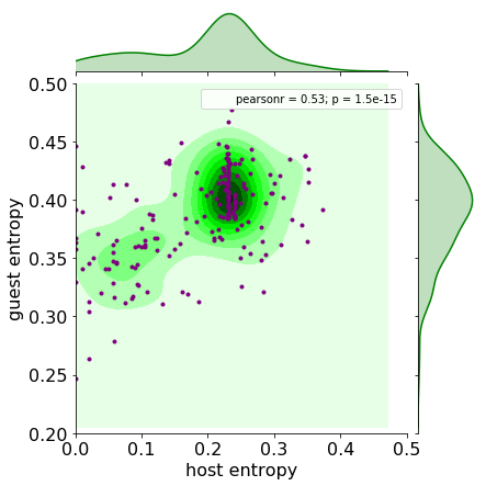
It is immediately seen that countries do not have random requirements, for the maximum entropy is around 0.4. On the contrary, each country is biased towards certain requirements. The guest entropy never hits its lower bound, indicating each country has at least two exit requirements. The countries whose host requirement is zero demand the same documents from all incoming citizens. There are around ten of them. However, the entropy does not state anything about the values of the random variate. A quick sorting (pun intended) tells which ones these are.
The statistics of the countries will be collected in the df_cnt_stats dataframe.
df_cnt_stats = pd.DataFrame({'code' : df_visa_clean.index})
df_cnt_stats['name'] = df_cnt_stats['code'].apply(lambda x: code_name_dict[x])
df_cnt_stats['guest_entropy'] = guest_entropy
df_cnt_stats[ 'host_entropy'] = host_entropy
df_cnt_stats['most_common_entry'] = [category_lookup[most_common(h)] for h in V.T]
df_cnt_stats['most_common_exit'] = [category_lookup[most_common(g)] for g in V]
# there is a weird bug in nsmallest and nlargest so we use sort_values instead
df_cnt_stats.sort_values(by=['host_entropy'])[['name', 'host_entropy', 'most_common_entry']].head(10)
| name | host_entropy | most_common_entry | |
|---|---|---|---|
| 57 | MICRONESIA | 0.000000 | visa-free |
| 111 | MADAGASCAR | 0.000000 | visa on arrival |
| 2 | AFGHANISTAN | 0.000000 | visa required |
| 121 | MALDIVES | 0.000000 | visa on arrival |
| 92 | NORTH KOREA | 0.000000 | visa required |
| 90 | COMOROS | 0.000000 | visa on arrival |
| 163 | SOMALIA | 0.000000 | visa on arrival |
| 44 | DJIBOUTI | 0.010582 | visa on arrival |
| 46 | DOMINICA | 0.010582 | visa-free |
| 154 | SEYCHELLES | 0.010582 | visa-free |
Indeed, uniform requirement for a country does not mean identical requirements across countries as we can see visa free, visa required and other categories.
Distribution of requirements
Host and guest scores
A crude estimation of how welcoming a country can be expressed as the mean of the her entry requirements. This will be called the host score, $s_{w}$.
\(s_{h}(i) = \frac{ \sum\limits_{j \neq i} v_{ji} } {n_{g} - 1}\) Likewise, the average of the exit requirements of a country will be called the guest score, $s_{g}$ and indicates how welcomed the citizens of that country are. \(s_{g}(i) = \frac{ \sum\limits_{j \neq i} v_{ij} } {n_{g} - 1}\)
sh = (V.sum(axis = 0) + 1) / (ng - 1)
sg = (V.sum(axis = 1) + 1) / (ng - 1)
The score distribution is shown below.
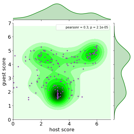
The histogram of the host and guest score plot hints at three major types of mutual relationships. Agglomerate of countries in the upper right corner indicates mutually restricted entry criteria. The bottom middle region of the graph groups countries that have mixed entry requirements but, in general, one can enter other countries reasonably easily. The top left cluster represents welcoming countries whose citizens face strict entry requirements.
Distribution of requirements
| The distribution of exit requirements i.e. documents required from a country, $\mathbf{p}{g}(i) \in \mathbb{R}^{n{g} \times | C | }$, i.e. histogram of the columns reflects how permissive a country is. |
pg = np.zeros((ng, nc))
count_gen = (np.unique(v, return_counts = True) for v in V)

for row, (idcs, count_) in zip(pg, count_gen): # blessed be passing references
    row[idcs[:-1]] = count_[:-1]

pg = pg / pg.sum(axis = 1)[:, None]
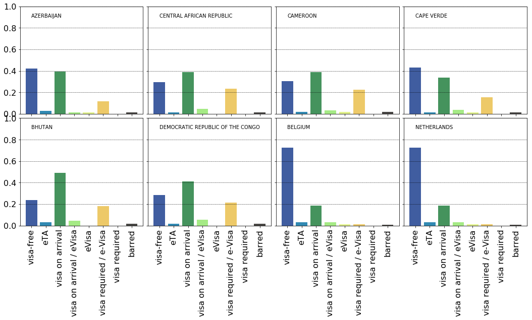
The distributions for Azerbaijan, Central African Republic, Cameroon, Cape Verde, Bhutan, DR Congo, Belgium and The Netherlands are show below. It is readily observed the first six countries are easier to travel from as to how much paperwork is needed compared to the last two ones. A question then naturally arises whether are there groups of countries of similar requirement patterns?
As a start, we can now easily figure out which country has the most polar exit requirements. The term ‘polar’ means separated bimodal distribution:
- there are two categories that are more likely than any other $\forall m \in C / {k, l} : p_{g}(i){k/l} > p{g}(i)_{m} $
- their probabilities are close to each other: $p_{g}(i){k} \approx p{g}(i)_{l}$
-
their separation is larger than half of the cardinality of the categories: $ k - l \geq \frac{ C }{2}$
A limiting case is where two categories have 0.5 and 0.5 probabilities. Based on the previous plots these categories are likely to be visa free, visa on arrival and visa required.
mask = np.zeros((3, nc), dtype = np.float)
mask[0,0] = mask[0,6] = 0.5           # visa free -- visa required
mask[1,0] = mask[1,2] = 0.5           # visa free -- visa on arrival
mask[2,2] = mask[2,6] = 0.5           # visa on arrival -- visa required
overlap = np.linalg.norm(pg[:,None,:] - mask, axis = 2)
bimodals = np.array([np.argsort(x)[:3] for x in overlap.T])
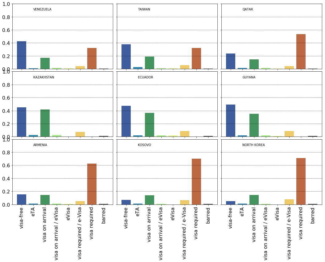
Each row of the plot above shows the three most polar distribution of requirements for the via free - visa required, visa free - visa on arrival and visa on arrival - visa required pairings.
Comparison of requirements
The distributions of the countries are compared via the Euclidean distance matrix, $D \in \mathcal{R}^{n_{g}\times n_{g}}$. \(d_{ij} = \| \mathbf{p}_{h}(i) - \mathbf{p}_{h}(j) \|^{2}_{2}\)
dist_mat = scd.squareform(scd.pdist(pg))
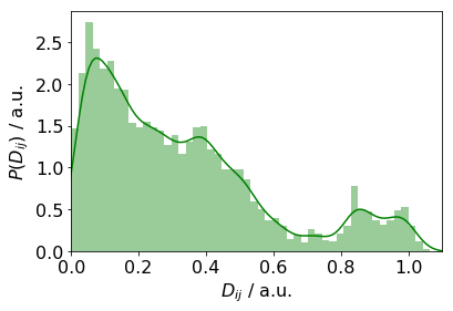
If there are $n$ clusters of similar $P_{g}$-s, then the maximum number of peaks in the distance plot is
$
\begin{equation}
\begin{pmatrix}
n
2
\end{pmatrix}
+ 1
\end{equation}
$.
There are about between 4 and 7 peaks in the plot above. This implies the number of clusters is 3 or 4. However, one cannot tell the which countries are in a certain cluster. In order to reveal this, we will group the $P_{g}(i)$ distributions for all countries. Firstly, we calculate the Ward linkage between the individual distributions. The number of clusters is then chosen. The following options are given:
- Perform a number of consecutive clusterings then choose the one where the intra cluster variance is below a certain limit with the maximum number of clusters.
- Calculate the linkage matrix, $Z$ and plot the inter cluster distance. The number of subgraphs to keep is deduced by the location from the largest gap between the successive inter cluster distances (see below).
- Calculate the linkage matrix and calculate the intra cluster distance in a breadth first traversal. Stop the traversal when the distance drops below a certain limit. This would save us from the computational burden of performing consecutive clustering thus assembling the same linkage matrix over and over again.
Z = linkage(pg, 'ward')
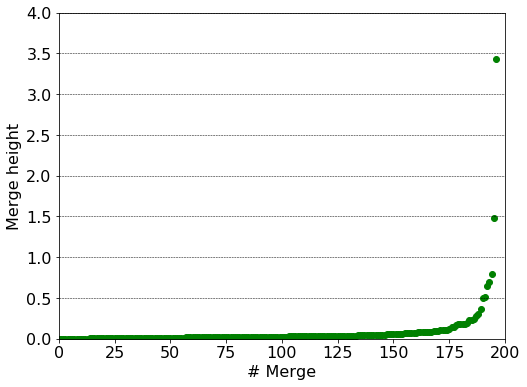
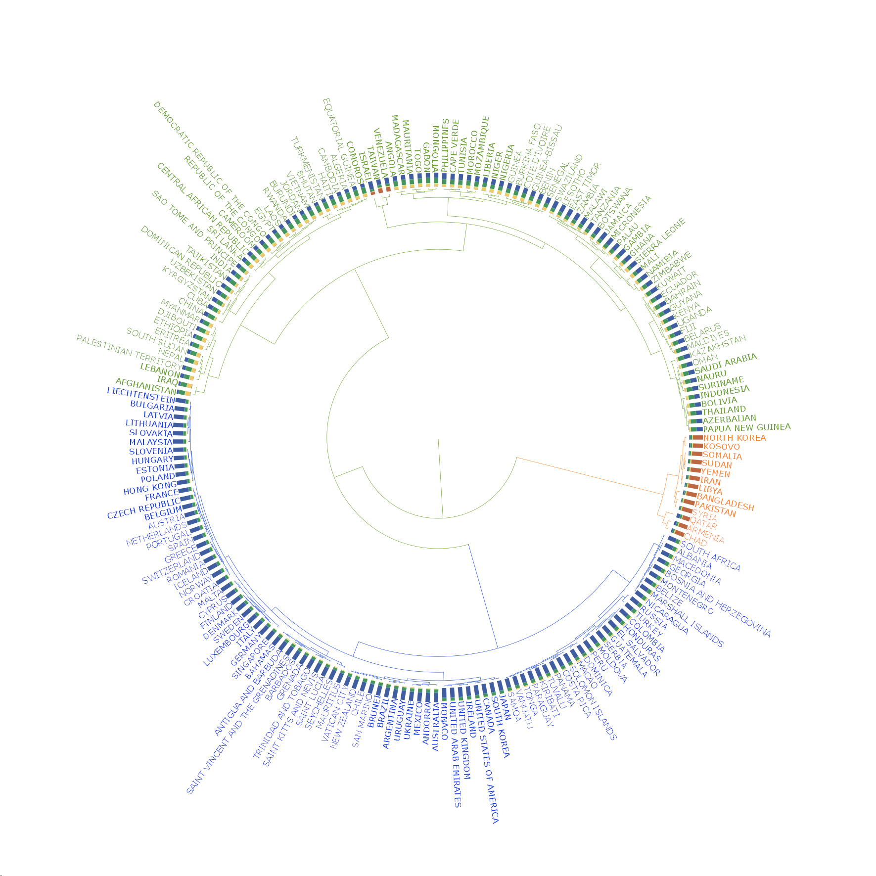
In the plot above each point corresponds to a merge. The merge height is also an upper bound for the intra cluster variance of the joined clusters. We therefore use method #1 to determine the number of clusters. The largest gap is between the penultimate point and the one before it, thus we will have three clusters.
In the following we create a circular dendrogram of the clusters.
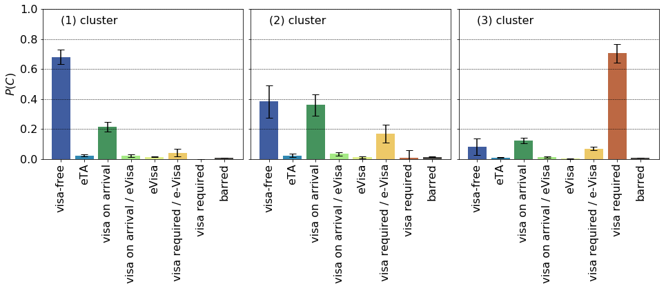
The dendrogram is split to three clusters:
clustaz = split_at_n_top(Z, 3)
The means and variance of the requirement distributions are then calculated:
means = np.array([np.mean(pg[_v], axis = 0) for _k, _v in clustaz.items()])
stds = np.array([np.std(pg[_v], axis = 0) for _k, _v in clustaz.items()])
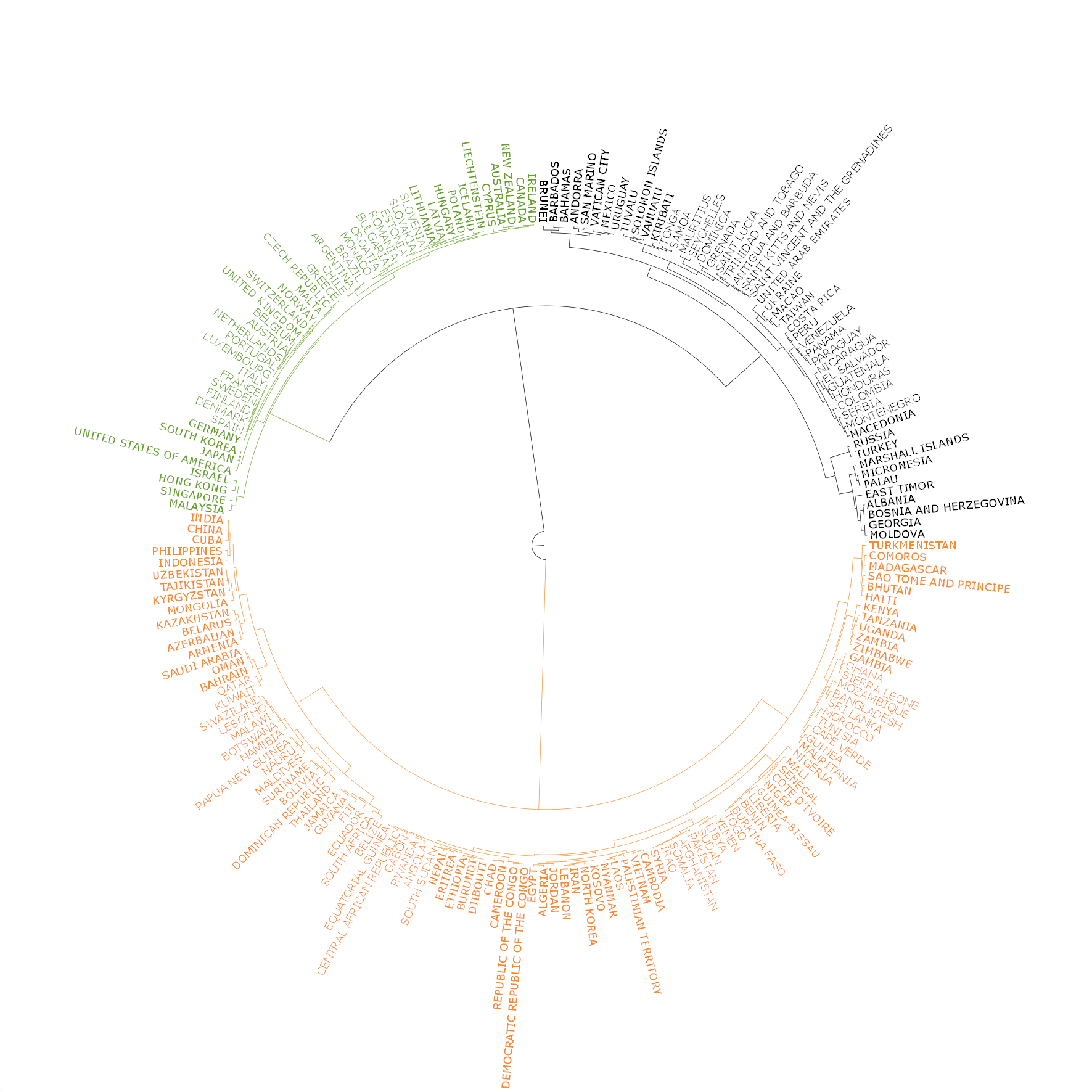
The three groups correspond to the most welcomed ones, e.g. as those in the EU, welcomed ones, such as many Asian and African countries. The third groups consists of countries with strained international relationships (Armenia) or ones with serious internal conflicts (Syria).
The dendrogram shows these clusters and the base distributions from which the distances were calculated, in anticlockwise order.
Mutual requirements
We turn our attention to the two way relationships ebodied in the requirements.
Reciprocity
Firstly, we investigate the reciprocity of requriments. To this end we pair, the $i \rightarrow j$ and $j \rightarrow i$ requirements and make a histogram of the pairs. The resulting matrix is called reciprocity matrix, $R$:
\[\begin{eqnarray} R & \in & \mathbb{N}^{|C| \times |C|} \\ r_{ij} & = & \sum\limits_{k<l} \delta(v_{kl}, c_{i}) \cdot \delta(v_{lk}, c_{j}) \end{eqnarray}\]tril = chain(*map(lambda x: zip(repeat(x-1, x), range(x)), range(ng, 1, -1))) # generator for lower triangle indices
recip_histo = Counter(map(lambda x: (V[x[1], x[0]], V[x[0], x[1]]), tril)) # count tuples
recip_mat = np.zeros((nc, nc), dtype = np.float) # convert to np.ndarray
for idcs, count_ in recip_histo.items():
recip_mat[idcs] = count_
recip_mat = recip_mat / np.sum(recip_mat)
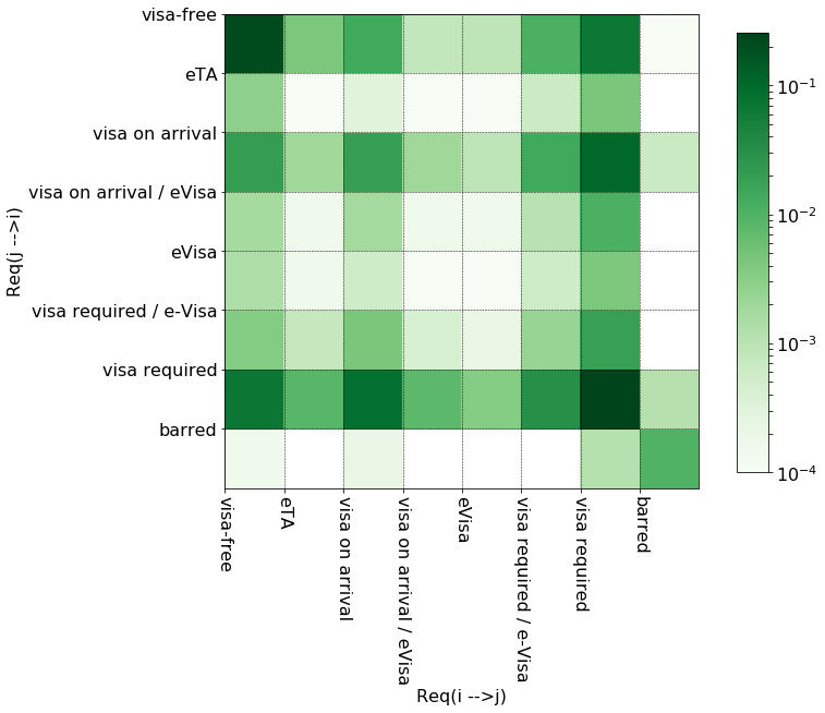
The matrix is not symmetric meaning that there are pairs of countries which demand different travel documents depending on the direction of travel. The most popular mutual requirements are
- (0,0) is the number of cases where entry from i to j is visa free and entry from j to i is visa free too
- (0,6) is the number of cases where entry from i to j is visa free and entry from j to i requires a visa
- likevise (6,0) is the number of cases where entry from i to j requires a visa and entry from j to i is visa free
- (2,6) and (6,2) are popular categories where visa on arrival is expected for a visa
The ratio of the identical requirements, r_req_iden is the trace of the matrix.
r_req_iden = np.trace(recip_mat)
print("Ratio of mutually identical entry requirements: {0:.4f}".format(r_req_iden))
Ratio of mutually identical entry requirements: 0.4997
Comparing countries by reciprocity patterns
In oder to compare individual countries, their reciprocity matrices, $R^{(k)} \in \mathbb{R}^{n_{c} \times n_{c}}$, have to be calculated.
\[r^{(i)}_{kl} = \frac{ \sum\limits_{j \neq i} \delta(c_{k},v_{ij}) \cdot \delta(c_{l}, v_{ji})} {n_{g} - 1}\]The reciprocity matrix, $R$ defined earlier is the sum of the individual reciprocity matrices:
\[R = \sum\limits_{i} R^{(i)}\]The few lines below conveniently do this job:
cnt_recip_mat = np.zeros((ng, nc, nc), dtype = np.float)

for idx, (g, h) in enumerate(zip(V, V.T)):                         # make pairs
    count_dict = dict(Counter(zip(g, h)))                          # count pairs of requirements
    _ = count_dict.pop((-1, -1), None)                             # remove (-1, -1) if present

    for (r, c), count_ in count_dict.items():                       # populate matrix
        cnt_recip_mat[idx, r, c] = count_

cnt_recip_mat = np.reshape(cnt_recip_mat, (ng, nc * nc))
normalize(cnt_recip_mat, norm = 'l1', axis = 1, copy = False);
A way to identify repeating patterns is to perform a PCA analysis. There are, however, two issues with PCA. Firstly, it only accounts for linear dependencies, secondly it only looks at linear transformation of the data. Nevertheless, it recovers some basic relationships.
pca = PCA();
pca.fit(cnt_recip_mat)
PCA(copy=True, iterated_power='auto', n_components=None, random_state=None,
  svd_solver='auto', tol=0.0, whiten=False)
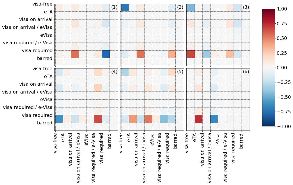
We are going to the first few principal components that account for the 95% of the total variance.
evr = pca.explained_variance_ratio_
cevr = np.cumsum(evr)
keep_idcs = np.arange(64, dtype = np.int)[cevr < 0.95]
print(keep_idcs)
[0 1 2 3 4 5]
Only six components are retained out of sixty four. It is inetersting to see that most of the linear relationships involve the visa required restriction. For example, the first component (top left corner) indicates that a pair of countries either has (visa required, visa on arrival) xor (visa required, visa required) mutual requirements.
Clustering
It would be interesting to see whether there are clusters formed around certain reciprocity patterns. First of all, a dissimilarity measure is needed. Taking the $L_{2}$ overlap of the reciprocity distributions can be misleading. For example, consider the following three distributions below:
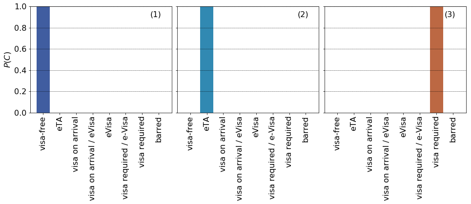
The $L_{p}$ distances between any two distributions are equal. However, we feel that (1) is closer to (2) than to (3) for visa free is closer to ETA than to visa required. In general, when comparing probability distributions over ordered categorical variables it is advantageous to use a distance that represets the underlying ordering. One such function is the earth mover’s distance (EMD) or Wasserstein metric. It is the minimum work required to move one distribution to match and other one, in a nutshell. Before we calculate EMDs for the countries two notes are in order:
- The two dimensional nature of the reciprocity matrix is taken into account by generating a 2D ground distance matrix. For the details please see
calc_ground_distance_2din the appendix. - The hiearchical clustering matches pairs of distributions with gradually increasing $L_{2}$ distance. As a consequence, the above effect is mitigated to some extent, for the widely dissimilar vectors are unlikely to be paired.
The ground distance matrix is calculated:
def calc_ground_distance_2D(N):
    """
    Calculates the 2D Manhattan distance for a N*N grid. It returns the flattened 2D distance matrix
    d(ij,kl) = |i - j| + |k - l| (4D)
    Let: m = i * N + j and n = k * N + l
    Let D \in N^{n^2, n^2}
    Then D(n,m) = d(n//N, mod(n,N), m//N, mod(m,N)) = d(ij, kl)
    Parameters:
        N (int) : gridsize
    Returns:
        dmat (np.ndarray[:,:] dtype = np.int) : the flattened Manhattan distance matrix
    """

    i_arr = np.repeat(np.arange(N, dtype = np.int), N)
    j_arr = np.tile(np.arange(N, dtype = np.int), N)

    dmat = np.abs(np.subtract.outer(i_arr,i_arr)) + np.abs(np.subtract.outer(j_arr, j_arr))

    return dmat
d_ground = calc_ground_distance_2D(8)
The matrix below is the ground distance between two flattened reciprocity matrix. The $(m,n)$-th element is the $L_{1}$ distance between
\[\big(i \leftarrow \lfloor \frac{m} {n_{c}} \rfloor, j \leftarrow \text{mod}(m, n_{c})\big) \text{ and } \big(k \leftarrow \lfloor \frac{n} {n_{c}} \rfloor, l \leftarrow \text{mod}(n, n_{c})\big)\]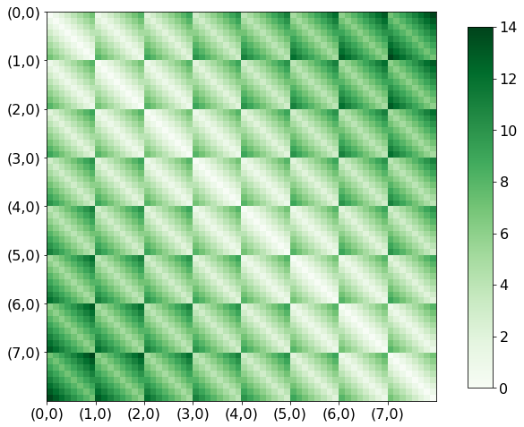
We can now calculate the EMD, emd, for all pairs of countries using the Python Optimal Transport module. We also calculate the Euclidean distance, l2d, for comparison.
import ot
emd = scd.squareform(scd.pdist(cnt_recip_mat, lambda x, y: ot.emd2(x, y, d_ground)))
l2d = scd.squareform(scd.pdist(cnt_recip_mat))
It is readily seen from the joint plot below that the earth mover’s distance is usually larger than the ordinary $L_{2}$ distance. This is due to taking the distance between the ordered categories into account.
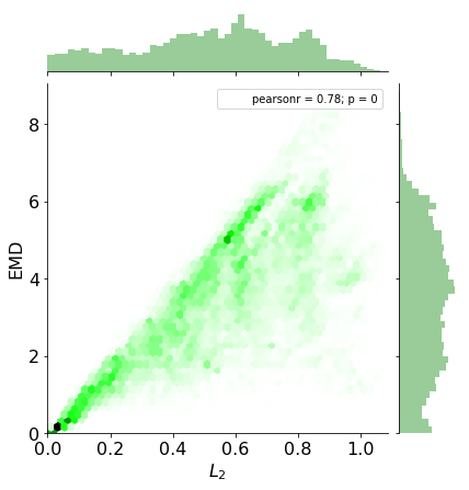
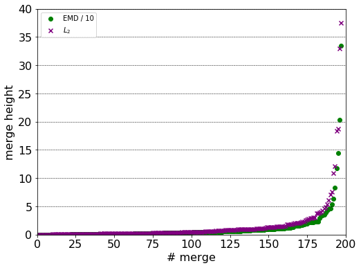
Two hierarchical clusterings are generated, one for EMD and one for $L_{2}$ distance.
Z_emd = linkage(emd, 'ward')
Z_l2d = linkage(l2d, 'ward')
The EMD is an order of magnitude larger than the $L_{2}$ distance, due to the underlying ground distance. The distribution of merge heights also differ. The $L_{2}$ metric generates are more branched structure at at larger heights.
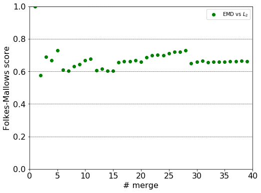
The labels in the top forty clusters are compared with respect to the induced Fowlkes-Mallows score. The closer its value to unit, the more labels can be found grouped in the same clusters in the two hierarchy.
label_pairs = ((linkage_to_labels(Z_emd, n), linkage_to_labels(Z_l2d, n)) for n in range(1,40))
scores = list(fowlkes_mallows_score(*lp) for lp in label_pairs)
The score is unit when all countries are in a single cluster as expected. It plummets just below 0.6 indicating the topmost merge partitions the countries quite differently. The next lower merges increase the value of the score, so that the countries within the top two clusters are grouped into similar clusters. This jaggedy behaviour is due to the EMD and $L_{2}$ distance being correlated. In case of two independent partitionings, the score is expected to monotonically decrease.
Back to the EMD clustering: where to cut the dendrogam? For there is no apparent gap (or elbow) in the succession of merge heights, the silhouette method will be invoked.
label_gen = (linkage_to_labels(Z_emd, n) for n in range(2,40))
score_gen = (silhouette_score(emd, label, metric = 'precomputed') for label in label_gen)
scores = np.fromiter(score_gen, dtype = np.float)

n_clusters = np.argmax(scores) + 2
print("Silhouette maximum at number of clusters: {0}".format(n_clusters))
Silhouette maximum at number of clusters: 5
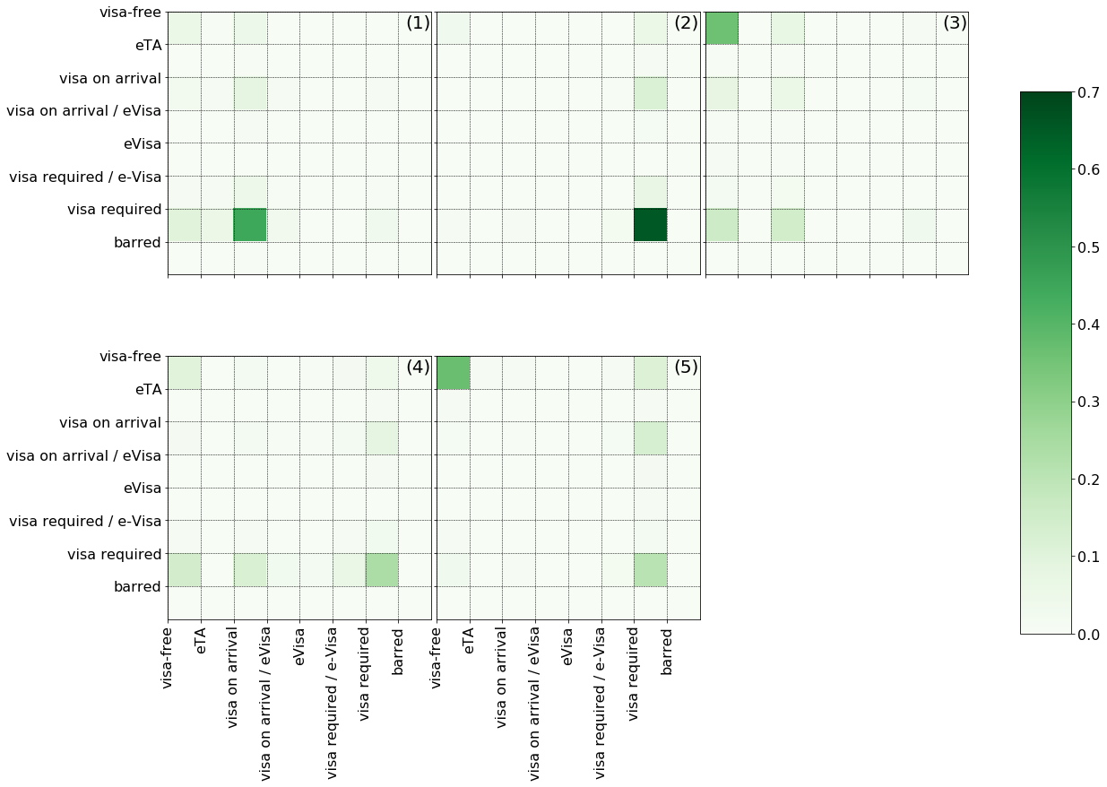
The tree thus will be cut to yield five clusters. The means of the reciprocity matrices within each cluster are shown below. The first three roughly corresponds to the (visa required, visa on arrival), (visa required, visa requiredl), (visa free, visa free) relationships. The fourth group collates countries that are less welcoming than welcomed. The fifth represents a group of countries which either have mutual visa free arrangements or being demanded visa required.
clustaz_ = split_at_n_top(Z_emd, 5)
means_ = np.array([np.mean(cnt_recip_mat[_v], axis = 0) for _k, _v in clustaz_.items()])
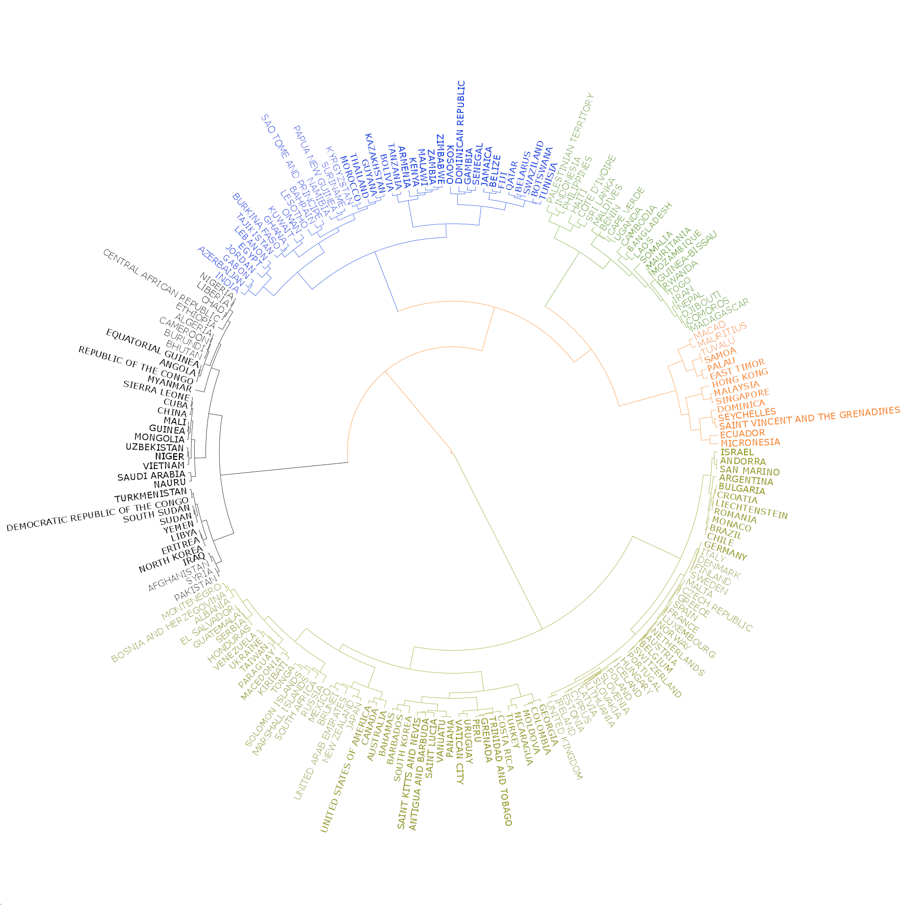
The dendrogram of the five clusters is shown below in anticloskwise order.
Asymmetry
Next, we calculate the conditional distribution of requirements with respect to the exit requirements. This is easily achieved by normalising each row of the overall reciprocity matrix.
p_recip_mat = recip_mat / np.sum(recip_mat, axis = 0)
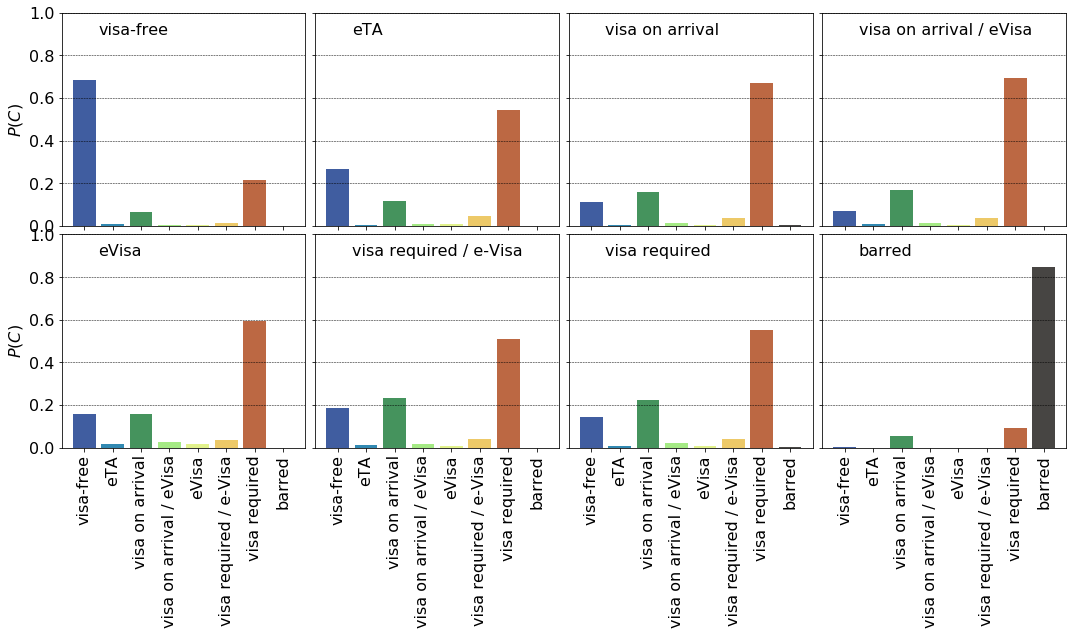
From these probability plots one can deduce that visa free and visa on arrival requirements are the mostly reciprocated ($p_{0,0}= 0.7, p_{7,7} = 0.55$). Countries also tend to mutually bar each other’s citizen’s ($p_{8,8} = 0.95$). At least there is something they agree on.
Quantifying reciprocity
To see much a country’s entry requirements reciprocated, the overlap between host $v_{i,}$ and guest $v_{,i}$ vectors is calculated.
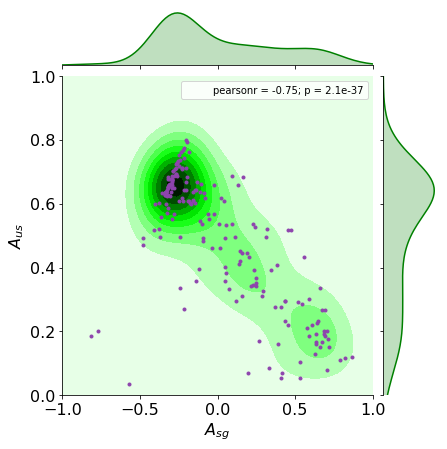
\[A_{us}(i) = \frac{\sum\limits_{k} \delta(v_{ik},v_{ki})}{n_{g}}\]A more sophisticated indicator is the count the sing of the differences, $A_{sg}$. Negative values are assigned to countries that are more welcoming than welcomed.
\[A_{sg} = \frac{\sum\limits_{k} \text{sign}(v_{ik} - v_{ki}) } {n_{g}}\]A third measure of asymmetry is the signed sum of differences, $A_{ss}$. However, the assignment of the actual numerical values to the categories, apart from being ordered, is somewhat accidental.
\[A_{ss} = \frac{\sum\limits_{k} v_{ik} - v_{ki} } {n_{g} \cdot (\max(C) - \min(c)) }\]# A_{us} -- unsigned overlap
a_unsigned = np.fromiter((np.sum(g == h) for g, h in zip(V, V.T)), count = ng, dtype = np.float) / ng
# A_{sg} -- signed difference
a_signed = np.fromiter((np.sum(np.sign(h - g)) for h, g in zip(V, V.T)), count = ng, dtype = np.float) / ng
# A_{ss} -- sum of signed difference
a_signed_sum = np.fromiter((np.sum(h - g) for h, g in zip(V, V.T)), count = ng, dtype = np.float) / ng / 7
df_cnt_stats['unsigned'] = a_unsigned
df_cnt_stats['signed'] = a_signed
df_cnt_stats['signed sum '] = a_signed_sum
The three most welcomed country:
df_cnt_stats.sort_values(by=['signed'])[['name', 'signed', 'unsigned']].head(3)
| name | signed | unsigned | |
|---|---|---|---|
| 186 | UNITED STATES OF AMERICA | -0.814070 | 0.185930 |
| 28 | CANADA | -0.768844 | 0.201005 |
| 9 | AUSTRALIA | -0.572864 | 0.035176 |
The three least welcomed countries:
df_cnt_stats.sort_values(by=['signed'])[['name', 'signed', 'unsigned']].tail(3)
| name | signed | unsigned | |
|---|---|---|---|
| 163 | SOMALIA | 0.788945 | 0.110553 |
| 33 | COTE D'IVOIRE | 0.824121 | 0.115578 |
| 73 | HAITI | 0.869347 | 0.120603 |
The sorted scores are shown below. The flatter regions indicate that numerous countries have similar asymmetric relations. However, looking at just $A_{us}$ and $A_{sg}$ does tell us whether the asymmetries of different signs compensate each other or a country has symmetric relationships.

A joint plot of $A_{us}$ and $A_{sg}$ can resolve this issue. The more asymmetric a country is the more likely it is more less welcomed then welcoming. These countries constitute top left cluster. If a country has symmetric relationships, ($A_{us}$) close to zero, it is likely to be less welcoming than welcomed according to the grouping in the bottom right corner.
Blocks
It is interesting to see whether there are groups of countries which have stronger ties among themselves than with others. An extreme example is a group where all entry requirements are visa free in both directions.
To this end consider the directed graph where the vertices are the countries; each of them connected by two directed edges corresponding to the entry requirements. We then color the edges according to their types e.g. Holy See and Italy are connected by two antiparallel blue edges. Finding a group of identical entry requirements is then equivalent to finding the n-cliques containing only edges of the same colour.
This can be done in the following way:
\[\begin{eqnarray} & & \textbf{Algorithm:} \textit{Find maximum disjoint coloured cliques} \\ &. & \quad \texttt{FMDCC}(G, c) \\ &. & \quad G' \leftarrow \left(V, G(E) \setminus \{v_{ij} \in G(E): \,\, \texttt{Colour}(v_{ij}) \neq \texttt{Colour}(v_{ji}) \} \right) \\ &. & \quad G' \leftarrow \left(V, G(E) \setminus \{v_{ij} \in G(E): \,\, \texttt{Colour}(v_{ij}) \neq c\} \right) \\ &. & \quad \mathbf{Blocks} \leftarrow () \\ &. & \quad \mathbb{S} \leftarrow \texttt{FindDisjointSubgraphs}(G') \\ &. & \quad \textbf{for} \,S \in \mathbb{S} \textbf{ do} \\ &. & \quad \quad \textbf{while} \, |S| > 0 \, \textbf{do} \\ &. & \quad \quad \quad C \leftarrow \texttt{FindMaximumClique}(S) \\ &. & \quad \quad \quad \mathbf{Blocks}.append( C) \\ &. & \quad \quad \quad S \leftarrow S \setminus C \\ &. & \quad \quad \textbf{end while} \\ &. & \quad \textbf{end do} \\ \end{eqnarray}\](To generate the plots below a fair of amount modestly interesting code is required. All of the functions can be found in the raw jupyter notebook.)
The cliques of visa free countries, cliques_vf are retrieved as:
cliques_vf = find_colour_max_cliques(V,0)
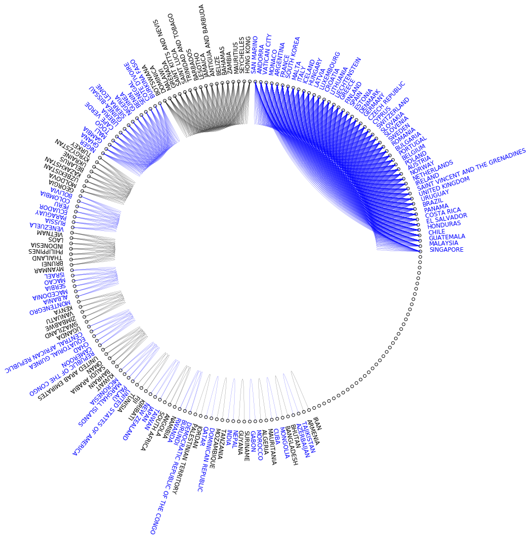
The blocks are then printed on a circular layout where each node correspond to a country, and each edge represents a mutual visa free requirement. Largest one consists of the Schengen/EEA/European microstates and numerous South American countries. Several Central American (plus a few African) states constitute the second largest group. The ECOWAS member states made up the third block. In general, countries of geopolitical proximity tend to form cliques. However, all connections in a clique should be visa free therefore even one asymmetric relationship can remove an otherwise perfectly connected country. A fine example is Russia, which requires visa from some of the Central Asian republics, therefore it is cannot be in the mainly post Soviet fourth block.
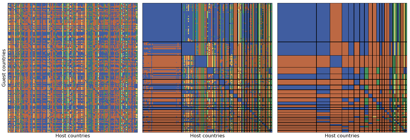
The original matrix, $V$ (1) shows no apparent structure. When countries are reordered, the blocks appear along the diagonal. Off-diagonal blocks can also be spotted where the requirements are dominated by a certain category. This is amplified is the mode of each block is plotted (c). The largest visa free clique comprises European and South American countries. Again, it is easier to travel from than to travel to these countries as the leftmost and topmost bands suggests.
Requirement similarity
Finally, we compare countries by their country specific requirements. Again, we start with defining a distance. The most straightforward choice is the simple matching coefficient, $d_{smc}$ excluding the host and guest countries:
\[d_{smc}(ij) = \sum\limits_{k\notin \{i,j\}} \delta ( v_{ik}, v_{jk}) \, .\]This, however, is not a proper metric and does not take into account the ordering of the categories. The second choice can be the $L_{1}$ distance, again excluding the host and gues countries:
\[d_{L1} = \sum\limits_{k\notin \{i,j\}} | v_{ik} - v_{jk} | \, .\]The drawback of this one, that the numerical values of the ordinal categories are arbitrary. One can use the Jaccard distance over the sets of tuples:
\[d_{Jac} = \frac{S_{i} \cap S_{j} } { S_{i} \cup S_{j} }\,\, \text{where } S_{k} = \{(k, v_{kl}) \},\,\, k\neq l\]We will use the $L_{1}$ distance, masked_l1, for it reflects the ordering of the categories which is then fed into a hierarchical Ward clustering.
def masked_l1(v1, v2, mask_value = -1):
    """
    Calculates the L1 distance between two arrays where all elements of specified value are masked.
    Parameters:
        v1, v2 (np.ndarray) : arrays to compare
        mask_value ({np.int, np.float}) : values to ignore
    Returns:
        l1 (np.float) : L1 distance
    """
    mask = (v1 != -1) & (v2 != -1)
    l1 = np.sum(np.abs(v1[mask] - v2[mask]))

    return l1
d_l1m = scd.squareform(scd.pdist(V, lambda x, y: masked_l1(x, y)))
Z_l1m = linkage(d_l1m, 'ward')
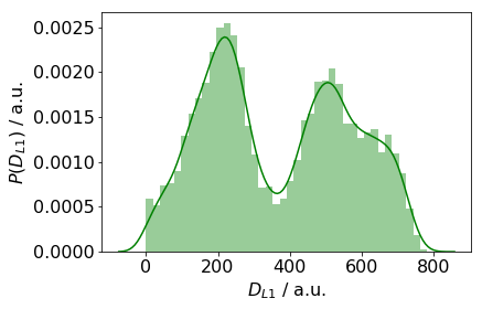
The histogram of the distances suggest there are at least three clusters (3*2 / 2).
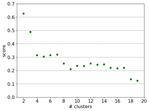
The silhouette index assumes it maximum at the topmost merge. However, we choose to add one more split which justified by the density plot above and the large gap between the second and third merges (between 3 and 4 clusters).
label_gen = (linkage_to_labels(Z_l1m, n) for n in range(2,20))
score_gen = (silhouette_score(d_l1m, label, metric = 'precomputed') for label in label_gen)
scores = np.fromiter(score_gen, dtype = np.float)
Again a geopolitical segmentation is readily observed most strikingly in the cases of post Soviet and African states.
