Aim
In this post we will investigate whether it is possible to predict cryptocurrency names based on known names.
Preliminaries
Modules
The following modules and tools will be needed:
from collections import Counter
from itertools import chain, islice, repeat
import json
import os.path

import matplotlib.pyplot as plt
import numpy as np
import pandas as pd

from sklearn.preprocessing import  normalize

from scipy.stats import chi2, chi2_contingency, poisson
import seaborn as sns
Data
The data have been collected from the crypocompare.com website.
Coding
Some of the functions have been moved to the Appendix. The raw notebook can be found here.
Coin list
The list of coins are loaded to the indeed creatively named coin_df dataframe.
coin_df = load_df_from_json(r'path/to/coin_attributes.json')
coin_df.head()
| Algorithm | CoinName | FullName | FullyPremined | Id | ImageUrl | IsTrading | Name | PreMinedValue | ProofType | SortOrder | Sponsored | Symbol | TotalCoinSupply | TotalCoinsFreeFloat | Url | |
|---|---|---|---|---|---|---|---|---|---|---|---|---|---|---|---|---|
| 42 | Scrypt | 42 Coin | 42 Coin (42) | 0 | 4321 | /media/12318415/42.png | 1 | 42 | N/A | PoW/PoS | 34 | 0 | 42 | 42 | N/A | /coins/42/overview |
| 300 | N/A | 300 token | 300 token (300) | 0 | 749869 | /media/27010595/300.png | 1 | 300 | N/A | N/A | 2212 | 0 | 300 | 300 | N/A | /coins/300/overview |
| 365 | X11 | 365Coin | 365Coin (365) | 0 | 33639 | /media/352070/365.png | 1 | 365 | N/A | PoW/PoS | 916 | 0 | 365 | 2300000000 | N/A | /coins/365/overview |
| 404 | Scrypt | 404Coin | 404Coin (404) | 0 | 21227 | /media/351001/404.png | 1 | 404 | N/A | PoW/PoS | 602 | 0 | 404 | 532000000 | N/A | /coins/404/overview |
| 611 | SHA256 | SixEleven | SixEleven (611) | 0 | 20909 | /media/350985/611.png | 1 | 611 | N/A | PoW | 586 | 0 | 611 | 611000 | N/A | /coins/611/overview |
Preparation
All names are cast as uppercase and any trailing whitespaces are removed. It is then checked whether there are missing names.
coin_df['clean_name'] = coin_df['CoinName'].apply(lambda x: x.strip().upper())

if coin_df['clean_name'].isnull().values.any():
    print("Warning: Missing name.")
else:
    print("No missing names")
No missing names
Analysis
Number of names and characters
Firstly, the number of names and characters are trivially determined, so that we know what sample size we are going to deal with. As we can see it is rather small. The corpus is usually in the order of hundred thousands or million words in common natural language processing setups.
n_name = coin_df['clean_name'].size
n_char = sum(map(lambda x: len(x), coin_df['clean_name']))
print("Number of names: {0}".format(n_name))
print("Number of characters: {0}".format(n_char))
Number of names: 2717
Number of characters: 25138
Character frequency
The character frequency yields a rough estimate of the name composition.
raw_char_frequency = Counter(chain(*coin_df['clean_name'].values))
n_letter = len(raw_char_frequency)
raw_chars, raw_freqs = zip(*raw_char_frequency.most_common())
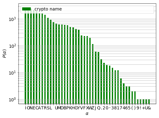
There is three orders of magnitude difference between the most and least frequent characters. (The gap between L and U is the space character.) Those names which contain any of the characters of frequency below a certain limit will be removed. This limit is twice the weighted square root of the top five frequencies.
n_top = 5
n_top_freq = np.array(raw_freqs[:n_top], dtype = np.float)
cutoff_freq = 2 * np.dot(np.sqrt(n_top_freq), n_top_freq) / np.sum(n_top_freq)

discard_chars, _  = zip(*filter(lambda x: x[1] < cutoff_freq, raw_char_frequency.items()))
names = list(filter(lambda x: not any(map(lambda y: y in x, discard_chars)), coin_df['clean_name']))
The selected names are then saved in the name_df dataframe. The number of names and characters are then quickly checked.
name_df = pd.DataFrame({'name' : names})
name_df['name_len'] = name_df['name'].apply(lambda x: len(x))
print("Number of names kept: {0}".format(name_df.shape[0]))
print("Number of characters kept: {0}".format(name_df['name_len'].sum()))
Number of names kept: 2489
Number of characters kept: 22997
The character frequencies and probabilities are calculated for the retained words and compared to the those if the original set.
char_frequency = Counter(chain(*names))
chars, freqs = zip(*char_frequency.most_common())

p_freqs = np.asarray(freqs, dtype = np.float) / sum(freqs)
r_raw_freqs = np.asarray(raw_freqs, dtype = np.float) / sum(raw_freqs)
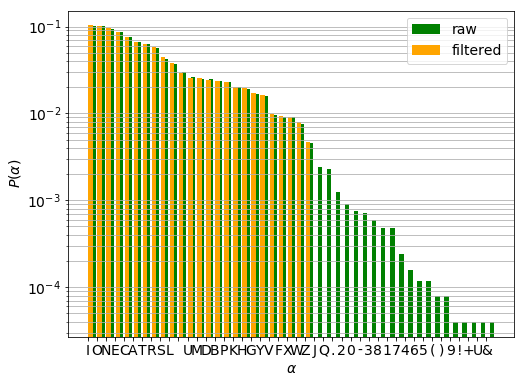
The distribution of characters that appear both in the raw and filtered sets are nearly identical which is confirmed by the $\chi^{2}$-test. It can thus be confirmed removing the words containing infrequent characters has not changed considerably our sample.
f_obs = np.asarray([freqs, raw_freqs[:len(freqs)]])
chi2_, p, dof, f_epx = chi2_contingency(f_obs)

print("P-value: {0}".format(p))
P-value: 0.999999997133692
Comparison to natural letter frequencies
It is interesting to compare the character frequency in the coin names to that of the English language. The reference distribution can be found here. They are loaded into a dictionary with letters as keys and the normalised frequencies as values.
with open('char_freq.json', 'r') as fproc:
    ref_letter_frequency = json.load(fproc)

ref_letter_frequency = {x.upper() : float(y) / 100.0 for x, y in ref_letter_frequency.items()}
The letter frequency of the names can easily be calculated, however, one has to make sure that only those letters are taken into account that appear in the reference list.
letter_frequency =  dict(filter(lambda x: x[0] in ref_letter_frequency, char_frequency.items()))

sum_ = sum(letter_frequency.values())
letter_frequency = {x : float(y) / sum_ for x, y in letter_frequency.items()}    # normalise

missing_letters = set(ref_letter_frequency.keys() - letter_frequency.keys())     # letters not in names
letter_frequency.update({x : 0 for x in missing_letters})
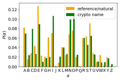
It is readily seen that the two distributions markedly differ.
Name length
If we assume there is a fixed average name length and the name lengths are distributed independently, we can try to model the length distribution with Poisson distribution. The exponent, the only parameter of the distribution is approximated by the mean of the observed word lengths.
name_len_histo = np.bincount(name_df['name_len'].values) * 1.0
name_len_histo /= max(1.0, np.sum(name_len_histo)) # dirty, I know -- but we also know that the lengths are 0< integers
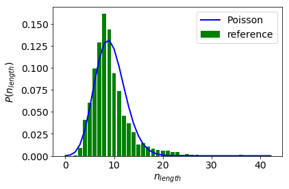
We can then perform a $\chi^{2}$-test on the Anscombe transformed data from which it can be established that the length distribution is not Poisson.
name_df['trf_vals'] = name_df['name_len'].apply(lambda x: np.sqrt(x + 0.375))
trf_vals = name_df['trf_vals'] - name_df['trf_vals'].sum()

chisq = np.dot(trf_vals,trf_vals)
print(chi2.sf(chisq, name_df.shape[0]))
0.0
Generating crytocurrency names
Our aim is to generate cryptocurrency names. The is a manifold of possible algorithms to achieve this. We are going to use a simple Markov model. We, therefore, have to know what what the probability of various character sequences across all coin names. The two letter sequences are counted below:
make_doublets = lambda x: zip(x[:-1], x[1:])
make_doublet_histo = lambda x: Counter(chain(*map(lambda x: make_doublets(x), x)))
pair_histo = make_doublet_histo(name_df['name'].values)
The overwhelming abundance of the word coin is readily recognised from the list of five most common sequences:
for pair, cnt in pair_histo.most_common(15):
    print("{0}\t:\t{1}".format(pair, cnt))
('I', 'N')	:	1246
('C', 'O')	:	1067
('O', 'I')	:	991
('E', 'N')	:	309
('E', 'R')	:	293
('I', 'T')	:	278
('T', 'O')	:	250
('R', 'E')	:	236
('A', 'R')	:	231
(' ', 'C')	:	215
('O', 'N')	:	197
('B', 'I')	:	190
('K', 'E')	:	187
('N', 'E')	:	184
('T', 'E')	:	167
The function counter_to_np_histo creates a 2D histogram of the character pairs. The rows correspond to the first character, whereas he columns hold the second character of every doublet. The additional keyword with_recorder returns the index $\rightarrow$ key element mapping.
The doublet histogram is then calculated:
histo, decoder = counter_to_np_array(pair_histo, with_decoder = True)
xlabels = ylabels = decoder.values()
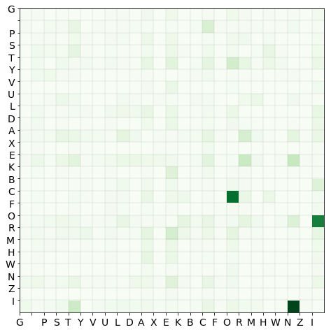
It is quickly checked whether any characters (a column and a row of the same index) can be removed. This would be the case if there are name that consist of a single character, and that character does not appear in any other names.
Other limiting cases:
- if a character is always terminal in all names it appears, its row is empty
- if a character is always the first one in all names it appears, its column will be empty
We can confirm that all characters are connected to at least one other character:
is_terminal = np.any(histo.sum(axis = 1) == 0.0)
is_starting = np.any(histo.sum(axis = 0) == 0.0)
is_standalone = is_terminal & is_starting

chooser = lambda x: 'yes' if x else 'No-o'

print("-Are there standalone characters? \n-The computer says {0}.".format(chooser(is_standalone)))
print("-Are there start only characters? \n-The computer says {0}.".format(chooser(is_starting)))
print("-Are there terminal only characters? \n-The computer says {0}.".format(chooser(is_terminal)))
-Are there standalone characters?
-The computer says No-o.
-Are there start only characters?
-The computer says No-o.
-Are there terminal only characters?
-The computer says No-o.
Transition probability matrix
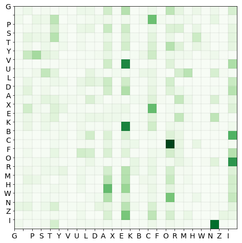
The row normalised histogram is the transition matrix $P$, tmat, where $P_{ij}$ is the probability that character $i$ is followed by character $j$.
Markov model
Under the assumption that a character is only determined by the preceding character, one can build a Markov model of the names. (We will see it is not a valid assumption later on.) The class MarkovSequenceGenerator creates a generator of Markov chain.
class MarkovSequenceGenerator(object):
    """
    Class to generate Markov sequences.

    Attributes:
        decoder ({int:object}) : dictionary that decodes the states
        encoder ({object:int}) : dictionary that assigns a unique index to every state
        transition_matrix (np.ndarray) : row normalised transition probability matrix

    Methods:
        create_sequence_generator (generator.object) : a generator which yields Markov sequences.
        Each returned item is a generator of a Markov sequence.
    """

    def __init__(self, transition_matrix, decoder, random_state = None):
        """
        transition_matrix (np.ndarray) : row normalised transition probability matrix
        decoder ({int:object}) : dictionary that decodes the states
        """

        self._decoder = decoder
        self._encoder = dict(zip(decoder.values(), decoder.keys()))
        self._transition_matrix = transition_matrix

        # calculate cumulative probabilities for sampling
        self.__cumprob_matrix = np.cumsum(self.transition_matrix, axis = 1)

    @property
    def decoder(self):
        return self._decoder

    @property
    def encoder(self):
        return self._encoder

    @property
    def transition_matrix(self):
        return self._transition_matrix

    def create_sequence_generator(self, start):
        """
        Creates a generator of a Markov sequence.
        Parameters:
            start (object) : starting state
        Returns:
            sequence_generator (generator) : a generator object of a Markov sequence
        """

        if start not in self.encoder.keys():
            raise KeyError("Start value not in known states. Got: {0}".format(start))

        self.__idx = self._encoder[start]

        def sequence_generator(start_index):
            """
            A Markov sequence.
                Returns the state at `start_index`
                Propagates the chain by one step.
            Parameters:
                start_index (int) : index of the starting Markov state.
            """

            idx = start_index

            while True:

                if idx is None:
                    return

                symbol = self._decoder[idx]
                idx = self._propagate_one_step(idx)

                yield symbol

        return sequence_generator(self.__idx)

    def _propagate_one_step(self, idx):
        """
        Propagates the Markov chain by one step.
        Parameters:
            idx (int) : index of the current Markov state.
        Returns:
            next_idx (int) or None: the index of the next Markov state. None if the chain ended.
        """

        x = np.random.rand()

        # nowhere to go
        if self.__cumprob_matrix[idx, -1] == 0.0:
            return
        else:
            next_idx = int(np.argwhere(self.__cumprob_matrix[idx] - x > 0.0)[0])

        return next_idx
Three random sequences are then generated.
msqg = MarkovSequenceGenerator(tmat, decoder)

n_seq_len = 50
seqs = (msqg.create_sequence_generator(start) for start in ['C', 'C', 'Y'])

for seq in seqs:
    print("".join(islice(seq, n_seq_len)))
COT INUKRDCENLE HARININDENERRBIBLLICTOIASHLOINENEL
COINCTINE NERTOIOAMENSTAINDOYPERCOINANDSTBENTARISP
YCKE EZEMALYPECUCRYWER BININOICOINN NECOINDERSTHEX
| The ‘C | O | I | N’ motiff can be recognised in all strings. These strings are infinite for there are no terminal only characters. In order to make them finite we have to modify our model. |
Start and terminating symbols
These continuous sequences reflect the probability of 2-long sequences in all of the original names. Our model bears little information on the distribution of starting and ending characters. Therefore the names are blended into each other.
This can be rectified by bracketing each original name with start and terminating symbols. Each of them will be prepended with the start symbol ’^’ appended by the terminating symbol ’$’.
start_symbol = '^'
end_symbol = '$'
name_df['aug_name'] = name_df['name'].apply(lambda x: start_symbol + x + end_symbol)
We can then calculate the transition matrix, now containing the delimiting characters, in the way we did previously:
# create histogram with decoder
pair_histo_aug = make_doublet_histo(name_df['aug_name'].values)
histo_aug, decoder_aug = counter_to_np_array(pair_histo_aug, with_decoder = True)

# transition matrix and labels
tmat_aug = normalize(histo_aug, norm = 'l1', axis = 1)
xlabels = ylabels = decoder_aug.values()
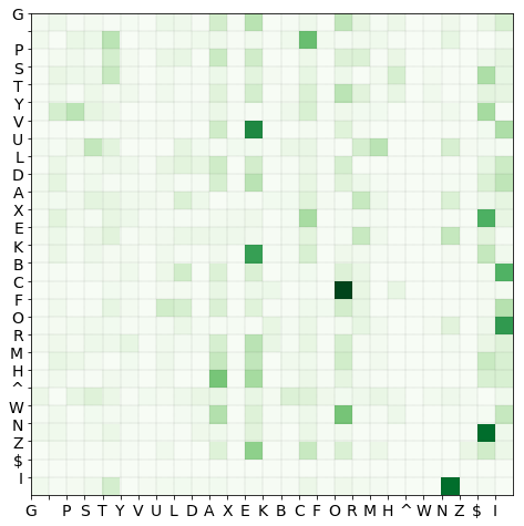
We then generate an infinite succession of Markov sequences which are themselves finite called seqs.
msqg_aug = MarkovSequenceGenerator(tmat_aug, decoder_aug)
seqs =  (msqg_aug.create_sequence_generator(x) for x in repeat(start_symbol))
Ten sequences are then consumed. Each of them corresponds to a generated cryptocurrency name.
n_seqs = 10
for idx, seq in enumerate(islice(seqs, n_seqs)):
    print(idx, "\t:\t", "".join(seq))
0 	:	 ^RINLBIN$
1 	:	 ^COITS$
2 	:	 ^KECOSY$
3 	:	 ^MITCOIAYM$
4 	:	 ^COIOTIN$
5 	:	 ^GRESANCENARSCO AL BUMBINGHOK$
6 	:	 ^LOCHEN$
7 	:	 ^VEN$
8 	:	 ^TOIUARTROLERARICHGON$
9 	:	 ^LEUN$
How good is our model?
First of all one has to define what goodness means. There is a plethora of properties that can be calculated for both the reference and generated sets. Some of them are expected to be identical, such as character and digram frequencies. Some of them e.g. name length distribution are not, for the Markov process has no information about its length.
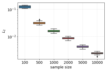
Firstly, we test the digram frequencies. The measure of goodness will be the L2 distance between the digram distributions. The overlap will depend on the sample size. Thus we use a succession of samples of increasing size to test this effect.
The population of generated words is called generated_words.
generated_words = np.asarray(["".join(seq) for seq in islice(seqs, 20000)])
sample_specs = {100 : 10, 500 : 10, 1000 : 10, 2000 : 10, 5000 : 10, 10000 : 10}
encoder_aug = dict(zip(decoder_aug.values(), decoder_aug.keys()))

sample_size_log, diff_log = [], []

for sample_size, repeats in sample_specs.items():

    for idx in range(repeats):
        # sample names and create transition matrix
        sample = np.random.choice(generated_words, size = sample_size)
        sample_histo = fill_np_array_with_counter(make_doublet_histo(sample), encoder_aug)

        # calculate difference
        diff = normalised_l2_diff(sample_histo, histo_aug)
        diff_log.append(diff)
        sample_size_log.append(sample_size)
The digram frequencies of the reference and generated names converge to each other as the sample size increases. At a sample size of 2000 the two distributions are practically identical
Name length distribution
Next, the length distributions of the reference and generated names are compared. The percentile bootstrap method is invoked to estimate the distributions and their confidence bands. A simple bootstrap algorithm is implemented in the SlimBootstrap class.
Firstly, the lengths of the generated names are calculated.
word_lengths = np.array([len(x) for x in generated_words])
max_len = np.max(word_lengths)
The bootstrap estimate and confidence bands are stored in the wl_dist array.
bins = np.arange(max_len + 1)
bstr = SlimBootstrap(func = sample_to_distribution, func_kwargs = {'bins' : bins})
wl_dist = bstr.fit_predict(word_lengths)
We then bootstrap the reference cryptocurrency names and compare the two distributions.
ref_word_lengths = name_df['name_len'].values
ref_bstr = SlimBootstrap(func = sample_to_distribution, func_kwargs = {'bins' : bins})
ref_wl_dist = bstr.fit_predict(ref_word_lengths)
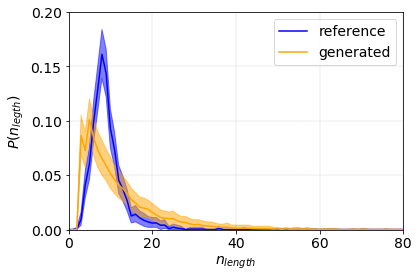
The two distributions markedly differ. The generated distribution is much wider and peaks at shorter lengths with respect to the reference one. This is due to the fact that the Markov model does not have memory. The probability that a sequence (a name) ends only depends on the probability of current character followed by the end symbol. It is independent of the absulute position of the current charachter.
This defect of the model can be mitigated by the inclusion of 3-grams, 4-grams etc in the Markov matrix. Also, one can design a recurrent neural network where the information on all to preceding characters are used with some weight.
Remarks
The goodness of fit warrants some further attention. Let us assume we have an alphabet $\Sigma$ whose Kleene star, $L$, contains every possible (existing or yet to be coined) crytocurrency names, $L_{c,all}$. The current selection of crytocurrency names, $L_{c}$, is a subset of all cryptocurrency names.
\[\begin{eqnarray} L &=& \Sigma^{*} \\ L_{c,all} &\subseteq & L \\ L_{c} & \subseteq & L_{c,all} \end{eqnarray}\]Our model can only use the alphabet $\Sigma$ and is required to produce words that are in $L$. The all possible generated names constitute the set $L_{g, all}$ which has a subset the realised names, $L_{g}$. One can think of the $L_{g, all}$ as all the Markov sequences, and $L_{g}$ as those are consumed.
\[\begin{eqnarray} L_{g,all} & \subseteq & L \\ L_{g} &\subseteq& L_{g,all} \end{eqnarray}\]Our aim is to write a model which maximises the $L_{g} \cap L_{c,all}$ intersection. It is immediately seen this task is ill-defined for the following issues:
- We do not know how the sizes of $L_{g}$ and $L_{g, all}$ compare. We therefore have to experiment at which sample size the fluctuations of its statistical properties of interest subdue to a sufficient level.
- We also do not know whether the properties of $L_{c}$ are true representatives those of $L_{c, all}$. We can only assume they are identical.
- The fluctuations of the properties of $L_{c}$ should also be estimated in order to determine to what extent to randomly selected not overlapping subset of $L_{c}$ are identical with respect to these properties. (i.e. if we train on a model on a subset, how well it is expected to perform.)
- As a consequence the goodness of the model can only be estimated by comparing the selected properties of $L_{g}$ and $L_{c}$.
In fact, this is exactly what we did when bootstrapped the reference and generated length distributions.
Appendix
These functions were used in the main body of the post. They deliver only a modest amount of excitement hence I moved them to the Appendix.
Functions to create and manipulate numpy histograms
def counter_to_np_array(counter, with_decoder = False):
    """
    Creates a numpy array based on a counter.
    Parameters:
        counter (collection.Counter) : a counter of length 2 keys
        with_decoder (bool) : if True returns a decoder dictionary. Default: False.
    Returns:
        array (np.ndarray) : 2D numpy array where each index corresponds to a key in counter.
        The value at a certain index is the corresponding count
        decoder ({:}) : a index : key dictionary if `with_decoder` is True
    """

    # key must be an iterable of length two
    key, count = counter.most_common(1)[0]
    key = list(key)

    if len(key) != 2:
        raise KeyError("counter key must be of length 2. Got: {0}".format(len(key)))

    # decompose to key count pairs
    keys, counts = counter.keys(), counter.values()

    # encode keys
    unique_symbols = set(chain(*keys))
    encoder = dict(zip(unique_symbols, range(len(unique_symbols))))
    xy = np.asarray([encoder[x] for x in chain(*keys)])
    xy = np.reshape(xy, (xy.shape[0] // 2, 2))

    # create histogram
    bins = np.arange(np.max(xy) + 2)
    weights = np.array(list(counts))
    array, _, _ = np.histogram2d(xy[:,0], xy[:,1], bins = [bins, bins], weights = weights)

    # add decoder if requested
    if with_decoder:
        decoder = dict(zip(encoder.values(), encoder.keys()))

        return array, decoder
    else:
        return array
def fill_np_array_with_counter(counter, encoder):
    """
    Fills a numpy array with a counter. It performs a *key --> *index transformation.
    Parameters:
        counter (collections.Counter) : a counter where all keys are of equal length.
        encoder ({}) : the keys are the keys of the counter (or a superset thereof) the values are integer indices.
    Returns:
        array (np.ndarray) : numpy array with counts.
    """

    n_size = len(encoder)
    mat = np.zeros(shape = (n_size, n_size), dtype = np.float)

    for (kx, ky), count in counter.items():
        mat[encoder[kx], encoder[ky]] = count

    return mat
Miscellaneous numeric functions
def normalised_l2_diff(p, q):
    """
    Calculates the normalised L2 difference between two arrays.
    Parameters:
        p (np.ndarray) : first distribution
        q (np.ndarray) : second distribution
    Returns:
        diff (np.float) : the L2 difference between the normalised p, and q distributions
    """

    p_ = normalize(p)
    q_ = normalize(q)

    denominator = (np.square(p_) + np.square(q_))
    if not np.any(denominator):
        raise ValueError("Both distributions are zero.")

    diff = np.sum(np.square(p_ - q_)) / np.sum(denominator)

    return diff
def sample_to_distribution(arr, *args, **kwargs):
    hist =  np.histogram(arr, *args, **kwargs)[0]

    sum_ = np.sum(hist)
    if sum_ == 0.0:
        hist = np.zeros(hist.shape)
    else:
        hist = hist * 1.0 / sum_

    return hist
Miscellaneous helper functions
def load_df_from_json(path_to_file, orient = 'index'):
    """
    Loads a pandas dataframe from a json file.
    Parameters:
        path_to_file (str) : **full** path to the json storage
        orient (str) : orientation of the json (see pandas.read_json for details)
    Returns:
        df (pandas.DataFrame) : a dataframe
    """
    with open(path_to_file, 'r') as fproc:
        df = pd.read_json(fproc, orient = orient)
    return df
Plotting functions
def plot_histomat(mat, ax = None, xlabels = None, ylabels = None):

    if ax is None:
        fig, ax = plt.subplots(1,1)
        fig.set_size_inches(8,8)

    n_xticks, n_yticks = mat.shape

    extent = (0, n_xticks, n_yticks, 0)

    ax.grid(color  = 'black', linestyle='--', linewidth = 0.1)

    ax.set_xticks(np.arange(n_xticks))
    ax.set_yticks(np.arange(n_yticks))

    if xlabels is not None:
        ax.set_xticklabels(xlabels)

    if ylabels is not None:
        ax.set_yticklabels(ylabels)

    ax.imshow(mat, extent = extent, cmap = 'Greens', vmin = 0)
Bootstrap class
class SlimBootstrap(object):
    """
    Simple percentile bootstrap class.
    Attributes:
        n_resample (int) : number of samples
        sample_size (int) : sample size -- number of elements taken from the population.
        alpha (float) : significance level at which the confidence interval is calculated

    Methods:
        fit() : calculates the percentile bootstrap estimate and confidence bands
        fit_predict() : returns the calculated estimate and confidence bands
    """

    def __init__(self, n_resample = 2000, sample_size = 1000, alpha = 0.05,
                 func = lambda x: x, func_args = [], func_kwargs = {}):
        """
        Parameters:
            n_resample (int) : number of samples. Default 2000.
            sample_size (int) : sample size -- number of elements taken from the population. Default 1000.
            alpha (float) : significance level at which the confidence interval is calculated. Default 0.05.
            func (callable) : function which is applied to the samples. The result of this function is bootstrapped.
                The bootstrap function can return any object as long as it can be cast to a regular np.ndarray.
                Default : identity function
            func_args ([]) : positional arguments of func. Default [].
            func_kwargs ({:}) : keyword arguments of func. Default {}.
        """

        self._n_resample = n_resample
        self._sample_size = sample_size
        self._alpha = alpha
        self._func = func
        self._func_args = func_args
        self._func_kwargs = func_kwargs

    @property
    def alpha(self):
        return self._alpha

    @property
    def n_resample(self):
        return self._n_resample

    @property
    def sample_size(self):
        return self._sample_size

    def _generate_samples(self):
        self.__samples = (np.random.choice(self.__population, self.sample_size)
                              for i in range(self.n_resample))

    def _set_population(self, population):
        self.__population = population

    def fit(self, population):
        """
        Calculates the bootstrap estimate and confidence bands.
        Parameters:
            population (indexable) : the population to be sampled.
        Returns:
            self
        Notes:
            The return values of the function are sorted along the first axis.
        """

        self._set_population(population)

        self._generate_samples()

        # 1) It would be better to apply the function to the entire population
        # simultaneously. However, it is not granted that the function is written that way.

        # 2) consume the generator here, so it can be cast as an array quicker
        measurements = list(self._func(x, *self._func_args, **self._func_kwargs)
                                for x in self.__samples)

        store = np.array(measurements)

        # sort in place along first axis
        store.sort(axis = -store.ndim)

        # bootstrap estimate
        estimate = np.mean(store, axis = -store.ndim)

        # confidence bands
        i_low = int(self._alpha / 2.0 * self._n_resample)
        i_up = int((1.0 - self._alpha / 2.0) * self._n_resample)

        cb_low = store[i_low]
        cb_up = store[i_up]

        self._result = np.array((estimate, cb_low, cb_up))

        return self

    def fit_predict(self, population):
        """
        Convenience wrapper around the `fit` method.
        Parameters:
            population (indexable) : population to be sampled
        Returns:
            self._result (np.ndarray) : the estimate and confidence bands
            _result[0] : estimate
            _result[1] : lower bound of confidence band
            _result[2] : upper bound of confidence band
        """
        return self.fit(population)._result