A simple mathematical formalism and a framework therein are presented to analyse recurring singles in the UK charts. We test this framework on the Christmas singles. It will also be shown that there is no trivial way to decide whether a single is intended to be a song for yuletide without using any information sourced from outside of the charts.
The raw notebook can be found here. The custom python utilities invoked in this post are stored at [this folder]((https://github.com/bhornung/bhornung.github.io/blob/master/assets/christmas-singles-1/scripts).
Prelude
I have been looking at the UK singes charts. In the first post the record labels were investigated. I set off to analyse the singles themselves. I loaded the data to a dataframe chart_df: Each single is encoded by a non-negative integer. As a quick check of the correctness of the encoding, the weekly mean codes were plotted. I deliberately chose the mean as a measure of consistency for it is sensitive to outliers. A monotonically increasing curve was expected. However, I got this:
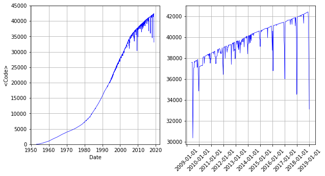
A curve with a trend of the right sign superimposed with seasonal downward spikes. These spikes appear around Christmas (see right panel above), which indicates they are due to recurring Christmas singles from the previous years. (A few searches in the database also confirmed this.) We therefore set out to investigate the Christmas singles (CS from now on) is this blog post.
Notation
A few useful definitions and notations are introduced which will be helpful in formalising the analysis.
Singles
A single is an ordered pair of song title and artist. The set of singles, $S$ is defined as
\[\mathcal{S} = \big\{ s_{k}, k \in \{1,..., N_{S}\} \big\}, \, \text{where} \\ 0 < N_{S}, \quad \text{(no-empty)} \\ \forall k,l, \, k \neq l : s_{k} \neq s_{l} \quad \text{(unique elements)}\]Chart
A chart of $0 < N_{W}$ weeks and $0 < N_{P}$ weekly positions is defined as
\[\mathbf{C} = \mathcal{S}^{N_{W} \times N_{P}} \quad \text{(rectangular matrix)}\\ \forall i,k : 0 \leq \bigg| \bigcup\limits_{j} \{c_{ij}\} \cap \{s_{k} \} \bigg| \leq 1 \quad \text{(a single can appear at most once in a week)}\]$C_{i,.}$ is the $i$- th week of the chart, whereas $C_{j}$ is the $j$-th position across the weeks.
The chart can also be interpreted as an indexed set with non-unique elements. We will heavily rely on this duality later on. Therefore, $C$ (single font) means the indexed set corresponding to the matrix chart $\mathbf{C}$.
Period
A period is a collection of subsequent rows (i.e. weeks) of the chart. A period is be denoted by $c_{[mn]}$ stretching from week $m$ to week $n$.
Slice
A slice is a collection of subsequent columns (i.e.) positions throughout all weeks. A slice between and including positions $m$ and $n$ is denoted by $c_{(mn)}$. It is often convenient to use the shorthand $i = [mn]$ to denote both slices and periods.
Selection
A selection is a submatrix (or subset) of the chart. It is the intersection of periods and slices.
Position
The position of the $s_{k}$ single in week $i$ in chart $C$, $v^{C}_{k,i}$ is defined as a result of a query:
\[v^{C}_{k,i} = \begin{cases} j, \quad & \text{if} \quad \big|\left\{ {j, 0 < j < N_{P}, j : c_{ij} = s_{k}} \right\}\big| = 1 \\ \text{undefined}, \quad &\text{if} \quad \big|\left\{ {j, 0 < j < N_{P}, j : c_{ij} = s_{k}} \right\}\big| = 0 \end{cases}\]There are no other cases for it has already been ensured that a single can appear at most once a week.
Time series of a single
A time series, history, progression of a single $s_{k}$ is defined as the succession of weeks and the associated weekly positions wherever the position is defined. Each point consists of the ordered pair of week, $i$ and the position $v^{U}_{k,i}$
\[\big((i, v^{C}_{k,i}) \big)_{i = i_{1}}^{i_{n}}, \, \quad \text{(pair of date and position)}\\ v^{C}_{k,i} \in \{1, ..., N_{P} \}, \, \quad \text{(defined)} \\ \forall k,l, \, \, k < l : i_{k} < i_{l} \, \quad \text{(ordered in time)}\]Christmas period
The Christmas period (CP) brackets the weeks immediately preceding and following the holiday. We define it as period of the chart falling on the subsequent months of December and January. The Christmas period starting in year $y$ is denoted by $C^{C}_{y}$.
Christmas single
We must define what constitutes a Christmas single. There are two approaches. The first one states that CS is a song that is usually played during multiple Christmas periods. These are easier to identify by looking for singles that appear in more than one CPs. This definition does not state anything about the origin of the song, or the original intent of the artists who produced it. The drawback of this definition that persistent singles that were not intended to be CSs will be accounted as those.
The second definition tries to capture the essence of the CSs. A CS is a song that was intended to be played during Christmas by creating an association between its features and the festive days. In general, it is not at all trivial to determine whether song is a CS just by inspecting the chart. They might only chart in a single year, or their timeseries can be indistinguishable from those of the non-CS singles.
The regretfully non-empty set of CS is denoted by $S_{C}$:
\[\mathcal{S_{C}} \subset \mathcal{S} \,.\]Recurring CS
A recurring CS, is a CS that appears in multiple CPs, or equivalently there are multiple $C^{C}{y}$-s in which a single appears. The set of recurring CSs are denoted by $S{CR}$
\[s_{k} \in S_{CR} \Leftrightarrow \big| \big\{ y \in \{1,..,N_{y}\}, s_{k} \in \mathcal{C}: s_{k} \in C^{C}_{y} \big\} \big| > 1\]The recurring Christmas singles constitute a subset of Christmas singles.
Useful notations
- non-unique set of singles in period $i$ is denoted by $c_{i}$.
- unique set of singles in period $i$ is denoted by $u_{i}$.
- unique set of single that first appeared in year $i$ is denoted by $f_{i}$
Notes
The number of weekly positions of the UK singles chart has changed over time, thus the actual chart is not rectangular. It is easy amend this by defining the missing data element $\epsilon$ and define the chart as $C = \big(S \cup {\epsilon} \big)^{N_{w}\times N_{P}}$.
Aim
We aim to answer two questions
- What is the prevalence of recurring Christmas singles?
- Is it worth to issue a Christmas single? (If you ask me, it is definitely not.)
We restrict our attention to recurring CSs which are possible to identify based on their chart positions without any knowledge about their textual or melodic properties.
Limitations
We will only investigate the top forty positions throughout the years. By doing so, the contamination from persistent non-Christmas singles is mitigated to some extent.
Analysis
Prevalence of outliers
Before we spend too much time answering these questions we should investigate how pronounced the recurrence of CS’s is. For this end, the overlap is calculated between all months.
The overlap, $o_{i,j}$ between periods $u^{i}$ and $u^{j}$ is defined as the number of singles present in both period divided by the number of singles of period which has fewer of them.
\[o_{ij} = \frac{ |c^{C}_{i} \cap c^{C}_{j}| }{\min(|c^{C}_{i}|, |c^{C}_{j}|)}\]The overlap is unit if one set is contained in the other, and zero if they have no elements/singles in common. Our (reasonably) efficient Tversky index algorithm will be used.
unique_in_months = chart_df.groupby((chart_df.index.year, chart_df.index.month)).apply(lambda x: np.unique(x.values.flat))

um = [np.array(x[x != -1], dtype = np.int32) for x in  unique_in_months.values]
overlap = calculate_pairwise_tversky(um, 1.0, 1.0)
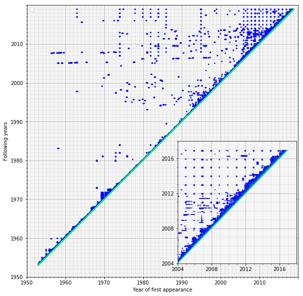
The overlap is plotted below.
- Each horizontal line shows the overlap with the charts from previous years.
- The diagonal is unit for each month totally overlaps with itself.
- The blue band above the diagonal is due to singles which chart for more than one consecutive months.
- The isolated dots signify singles which disappear from the charts for some time then reappear.
- These singles constitute a grid that falls on the Decembers.
- It is worth noting, the apparent lifetime of singles radically increases after 2000. We will investigate this phenomenon elsewhere.
Characteristics of recurrent Christmas singles
We defined the recurring Christmas singles as those singles which appear in multiple Christmas periods. They can easily be selected by forming the union of all intersections of unique singles in each Christmas period.
Number
\[S_{CR} = \bigcup\limits_{i<j} u^{C}_{i} \cap u^{C}_{j}\]The number of recurring CSs is surprisingly small being 56.
Contamination
There are two issues with the current definition:
- we are blind (unfortunately, not deaf) to CSs which only appear in a single period
- singles can persist for year or more in the charts. It could be that a non-CS (NCS) appear in multiple CPs therefore it is accounted as a CS.
In order to gauge the latter effect the charts are decomposed to CSs and NCSs. They are separated the chart_xmas_df and chart_nx_df dataframes, respectively. The 2D overlap graphs, along with the histogram of overlaps are shown below.
# select December and January
xmas_mask = (chart_df.index.month == 12) | (chart_df.index.month == 1)

# group December with following January
xmas_grouper = lambda x: x.year - 1953 + x.month // 12

# xmas singles
chart_xmas_df = chart_df.loc[xmas_mask]

# non xmas singles
chart_nx_df = chart_df.loc[~xmas_mask]
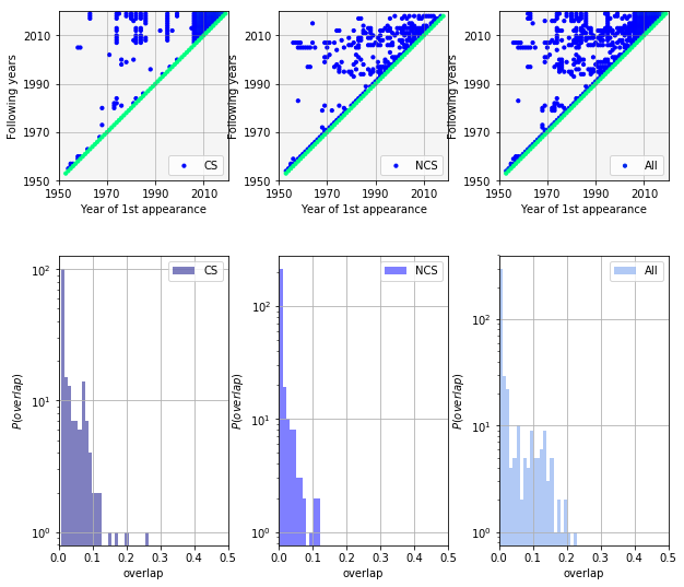
The overlap plots are different. The CS one has a grid-like structure, whilst the NCS plot is more random. The overlap plot of all singles is the weighted average of the previous two. Ideally, the NCS overlap would be zero, or much smaller than the overlap between CSs. The histograms show it otherwise. This is a potential issue, for the CSs are likely to be contaminated with recurring non Christmas singles.
Nevertheless, we proceed to develop a framework to analyse Christmas singles. The following machinery, in itself, does not depend on the definition of CSs, therefore it can be transferred to a scenario where the set of CSs are delineated more carefully.
Statistics by years
We develop a handful of measures to quantify the similarity and prevalence of singles. The term “year” will refer to the Christmas period of a year in the following.
Let,
-
$ c^{C}_{i} = N^{p}_{i}$, the number of positions in year $i$. -
$ f^{C}_{i} = N^{u}_{i}$ the number of unique labels in year $i$. - $n^{p}_{ij}$ the number of positions taken up singles which first appeared in year $j$, in year $i$.
- $n^{u}_{ij}$ the number of unique singles which first appeared in year $j$, in year $i$.
Retrospective or backward looking statistics
The probability that a single is from year $j$ given the year is $i$ is equal to:
\[P_{B}(j | i) = \frac{n^{p}_{ij}}{N^{P}_{i}}, \quad j < i\]The cumulative probability reflects how strong absorber of past singles a particular year is:
\[F_{B}(i) = P(j<i|i) = \sum\limits_{i<j} \frac{n^{p}_{ij}}{N^{p}_{i}}\]Similar probabilities can also be derived using the counts of the unique singles.
Forward looking statistics
There are two potential types of measures.
Overlap
The probability that a single first issued and selected from year $i$ appear in year $j$ is equal to:
\[P_{U}(j | i) = \frac{n^{u}_{ji}} {N^{u}_{i}}, \quad i < j\]The cumulative probability would show what is the likelihood that a single first appeared in year $i$ reappears in any of the following year. It is not possible to calculate this quantity given only the counts and it is of modes interest.
Coverage
The other forward looking aspect measures how strongly a year contribute to the charts in the following years. The probability that a single is from year $i$ given the year is $j$ is equal to:
\[P_{F}(j | i) = \frac{n^{p}_{ji}}{N^{p}_{j}}, \quad i < j\]The cumulative probability tells us how strong emitter a certain year is:
\[F_{F}(i) = P_{F}(i < j|i) = \sum\limits_{j<i} \frac{n^{p}_{ji}}{N^{p}_{j}}\]Using $F_{B}$ and $F_{F}$ one can tell how strong absorber or emitter a year is. The density functions, $P_{B}$, $P_{F}$ can be invoked to establish the degree of various types of similarities between years.
The backward and forward cumulative number ratios are shown below.
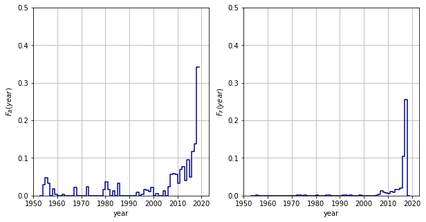
The ratio of the singles issued in preceding years are shown in the let panel.
- maximum 5% of the positions are populated by old singles for the first five decades
- after 2000, this ratio dramatically increases, perhaps, due to, background NCS singles
The forward statistics looks as expected.
- the probability that an early single covers large swathes of the future positions is negligible
- in the present decade, there is a large contribution from singles from the preceding years.
Single network
The backward looking probability distribution function, $P_{B}$, spans a graph.
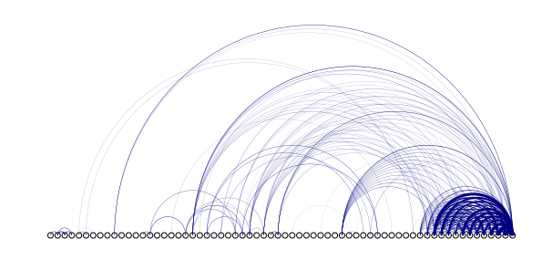
| Each black circle corresponds to a year. If a singe appeared in year $i$ and recharted in year $j$ a blue arc connects the two years. The width of which is proportional to the contribution to year $j$, $(P_{B}(j | i))$. Arcs are not drawn between two reappearances. Plus points are awarded for identifying “Rocking around the Christmas tree” and “Do they know it’s Christmas?”. |
Years of similar taste
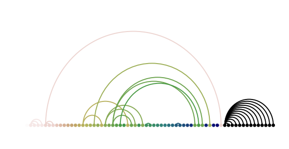
Expanding on the idea of the graph representation, one can create a network of years based on how similar their respective charts are. There is a plethora of similarity measures. We choose to gauge similarity by the normalised intersection of two non-unique sets:
\[= \frac{|u^{C}_{i} \cap u^{C}_{j}|} {|u^{C}_{i} \cup u^{C}_{j}|},\]which is the weighted Jaccard index of two charts. Arcs are now drawn between reappearances.

Clustering years
A logical next step is to group years by their similarities. We are going to use a Markov cluster algorithm. Each group of years coloured by the same colour have similar charts.
from MCAsparse.MCAsparse import MCsparse
from scipy.sparse import coo_matrix

# prepare distance matrix
jaccard = calculate_weighted_jaccard(xmas_numbers, with_diag = True)
X = coo_matrix((jaccard[2], (jaccard[0].astype(np.int32), jaccard[1].astype(np.int32)))).tocsr()

clusterer = MCsparse(inflate_power = 1.111, max_iter = 100, save_steps= True)
labels = clusterer.fit_predict(X)
Grouping of singles
Each edge in the graph above corresponds to a set of singles. Clustering the years by a similarity measure induces a clustering of singles.
Positions
An descriptive quantifier of the performance is the position. It is trivial to query the position of the Christmas singles, hence it is omitted from this discussion.
Summary
We have created a simple mathematical formalism and a framework composed of the components thereof to analyse recurring singles. We could only approximately identify the set of Christmas singles, due to persistent non Christmas singles.
Future work
In the next post digressing this topic, we develop two methods to find true Christmas singles. A careful analysis will also be carried out in the realm of the framework that we have developed.