Introduction
The topological features of the flags are investigated in this post. We will use it to uncover the various families of canvas designs.
Data
Raster images
We will use high resolution png images throughout this log post. They were obtained from pdf images as detailed in the previous post.
Image preprocessing
The coat of arms have been replaced by a uniformly coloured area in each flag to reduce complexity. Some flags were further modified:
- the Nepalese flag was stretched out to have a rectangular shape. This transformation does not affect its topology.
- The sun and its twelve rays were merged to one continuous object in the Taiwanese flag.
- The number of starts was reduced to five in the US flag,
Coding
As usual, only the relevant snippets of code are shared in this blog post. The raw notebook can be found here. The longer scripts are stored in this folder.
Preliminaries
Country codes
Each country is identfied through its two letter code.
with open(os.path.join(folder_lookup, "iso-country.json")) as fp:
    ccodes = json.load(fp)
Loading images
The images are loaded through a generator to avoid keeping large amount of data in the memory.
def create_image_loader(folder, func, tokens, ext):
    """Creates a generator of generator of images."""
    while True:
        gen_path = ((x, os.path.join(folder, f"{x}.{ext}")) for x in tokens)
        generator = ((k, func(v)) for k, v in gen_path)
        yield generator
An image loader is created straight away:
loader = create_image_loader(folder_simplified, imread, ccodes.keys(), "png")
Encoding
We are only interested in whether two colours are indentical or not irrespective the actual value of the colours themselves. The RGB colours are thus mapped to a field of one byte label for each flag.
def label_encode_image(image):
    """Returns an array of colour indices."""

    records = np.ascontiguousarray(image)\
              .view(np.dtype((np.void,
              image.dtype.itemsize * image.shape[-1])))

    labels, idcs = np.unique(records, return_inverse=True)
    image_new = idcs.reshape(image.shape[:2]).astype(np.uint8)

    return image_new
Results
A number of graphs will be created for each country. These will be stored in a central object, the connectivity dictionary.
connectivity = {}
Inner connectivity
Segments and connection
Each continuous region of the same colour is a segment. Each flag can be decomposed to a collection of segments. Two segments are connected is there is a section of finite length along which they touch each other. The way they are connected to each other defines the topology of a flag.
Implementation
Connected component labeling – image segmentation
An image is segmented in a one-sweep breadth first search. The algorithm array-segmenter iterates over the pixels of an image. The colours in a pixel’s four-neighbourhood are compared to the central colour. If any matches its label is set to that of the central pixel and it is added to the queue.
The array_segmenter algorithm returns an image where each segment has a unique label. It performs am exhaustive breadth first search over the pixels.
@nb.jit(nopython=True)
def array_segmenter(image):
    """Labels the connected components in a 2D image"""

    #
    im = image + 0
    nh, nw = im.shape[:2]

    not_found = False
    segment_counter = 0
    next_starts = [[nh//4, nw//4]]

    while np.any(im > -1):

        # get new i, j
        ii, jj = np.nonzero(im > -1)

        if len(ii) == 0:
            break
        else:
            i, j = ii[0], jj[0]
            queue = [[i, j]]
            active = im[i, j]

        segment_counter -= 1
        im[i, j] = segment_counter

        while len(queue) != 0:

            i, j = queue.pop()

            nbs = [(i-1, j), (i+1, j), (i, j-1), (i, j+1)]

            for k, l in nbs:
                if (-1 < k  < nh) and (-1 < l < nw):
                    if im[k, l] == active:
                        im[k, l] = segment_counter
                        queue.append([k, l])

    # flip sign
    im *= -1

    # shift to zero
    im -= 1

    return im
Determining connectivity between segments
The horizontal and vertical borders are determined. The labels are read from each side of the borders from which pairs are created. The components of these pairs are order to avoid creating duplicates. Finally, a set of pairs is formed which containes the connectivity information between segments. The result is a connecivity graph of the segments.
def get_segment_connectivity(image):
    """
    Determines the connectivity between image segments.
    """

    # horizontal borders
    i, j = np.nonzero(np.diff(image, axis=1))
    connectivity = set(zip(image[i, j], image[i, j+1]))

    # vertical borders
    i, j = np.nonzero(np.diff(image, axis=0))
    connectivity |= set(zip(image[i, j], image[i + 1, j]))

    # remove duplicates
    connectivity = set((min(x), max(x)) for x in connectivity)

    return connectivity
Processing
The images are loaded, encoded, segmented and the connectivity thereof is determined.
encoded = ((k, label_encode_image(v)) for k, v in next(loader))
segmented = ((k, array_segmenter(v)) for k, v in encoded)

connectivity["segments"] = {
    k: get_segment_connectivity(v)
    for k, v in segmented
}
Analysis
The raw output looks as follows:
sel = ["FR", "LU", "BF",  "PL", "CH"]

for k in sel:
    print(f"Connectivity of {ccodes[k]}: {connectivity['segments'][k]}")
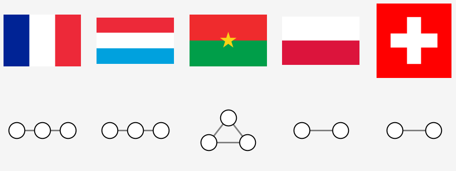
Connectivity of FRANCE: {(0, 1), (1, 2)}
Connectivity of LUXEMBOURG: {(0, 1), (1, 2)}
Connectivity of BURKINA FASO: {(0, 1), (0, 2), (1, 2)}
Connectivity of POLAND: {(0, 1)}
Connectivity of SWITZERLAND: {(0, 1)}
The flags of France and Luxembourg and Burkina Faso have three segments: 0, 1, 2. One connects to two and two connects to one. The Swiss flag is composed of two regions 0, 1 which are connected to each other. Just like the polish flag. As we can see, the topology is insensitive to the orientation of the flag.
Border region
The Polish and Swiss flags have the same topological representation. However, one might argue that they are different in a topological sense for the white area is enclosed by the red one in the latter one. This ambiguity can be resolved by adding a border region which skirts an entire flag. Only one area, the outer one, would be connected to this new region, whilst the inner one remains only attached to the outer one.
Implementation
The get_border_connectivity function screens along the one pixel wide edges of a flag and creates links to the border region will have the label -1.
def get_border_connectivity(image, single_region=True):
    """
    Determines the connectivity to the border region of a flag.
    """

    vals = (
        [-1, -3, -5, -7],
        [-1, -1, -1, -1]
    )[single_region]

    slices = ((0, ...), (-1,...), (..., 0), (..., -1))
    borders = (_get_padded_array_set(image[x], v) for x, v in zip(slices, vals))
    connectivity = reduce(set().union, borders)

    return connectivity


def _get_padded_array_set(x, val):
    """
    Creates a set of label tuples.
    """
    return set((val, x) for x in np.unique(x))
The inner and border connectivities are calculated in one sweep and then merged:
encoded = ((k, label_encode_image(v)) for k, v in next(loader))

# segment images
segmented = ((k, array_segmenter(v)) for k, v in encoded)

# calculate the two type of connectivities
connectivity["single-border"] = {
    k: (
        get_segment_connectivity(v),  # inside image
        get_border_connectivity(v)    # connectivity with the border
    )
    for k, v in segmented
}

# merge the two connectivities
connectivity["single-border"] = {
    k: v[0].union(v[1])
    for k, v in connectivity["single-border"].items()
}
Analysis
The same flags along with their representations are replotted. Two singly linked nodes appear now under the Swiss flag which clearly distinguishes it from the graph plot of Poland. The latter one forms a triangle.
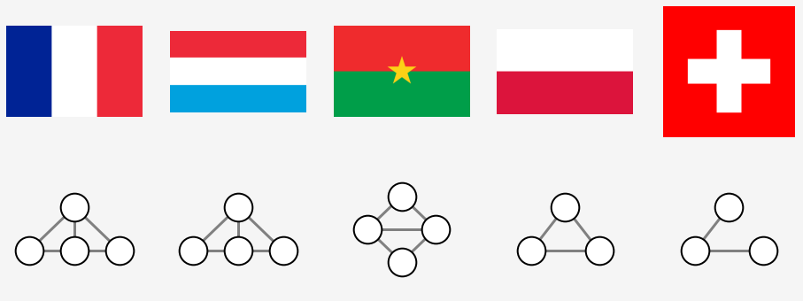
The following can be deduced
- enclaves without enclaves inside of them represented as a single node
- the outer region cannot be distinguished from the segments
The second point leads to ambiguity again. The topological plots of France, Luxembourg and Burkina Faso are identical, despite their topology being different. There are two ways to resolve this issue
- using directed graphs where and edge is drawn from the outer region to the inner one
- graph colouring where the node corresponding to the outer region is coloured differently to those marking the segments.
The first approach implicitly includes the second one, for the node index of the outer region needs to be known in advance in order to draw the edges. We therefore proceed to colour the nodes in the following.

The coloured graphs are now different for each flag as expected.
Isomorphism
A graph is isomorphic to an other if it is possible to relabel its nodes to create a one-to-one mapping between its nodes and edges and those of the second graph. As such, it is an excellent tool to groups topologically identical flags.
Isomorphism rule
Two nodes are considered identical if they are both segment nodes or border nodes.
Implementation
We are going to invoke the GraphMatcher function of the networkx package. Firstly, we need a function that adds a flag to each node indicating whether it is a segment node or not.
def label_nodes_single(g):
    """
    In place labeling of nodes.
    + 1: segment node
    - 1: border node
    """
    attr = {k: {"sg": copysign(1, k)} for k in g.nodes}
    nx.set_node_attributes(g, attr)
Secondly, a function is created which decides whether two nodes are of the same type.
def match_node_type_single(attr1, attr2):
    """
    Decides whether two nodes are of the same type.
    """
    res = 0 < (attr1["sg"] * attr2["sg"])
    return res
The labeled graphs are then created.
graphs = [(k, nx.from_edgelist(v)) for k, v in connectivity["single-border"].items()]
gen = (label_nodes_single(v) for k, v in graphs)
_ = reduce(lambda x, y: None, gen)
It is rather expensive to compute the graph isomorphish. Henceforth a number of shortcuts are introduced:
- We only iterate over the diagonal and upper triangle of the pairings.
- Isomorphism is transitive. If graph has already been assigned to a class, it needs no further comparisons.
- If two graphs have different number of nodes, they cannot be isomorph.
classes = defaultdict(set)
for i, (k1, g1) in enumerate(graphs):

    # isomorphism is transitive
    if any(k1 in v for v in classes.values()):
        continue

    for k2, g2 in graphs[i:]:

        # if it has not been found, it is in its own class
        if k1 == k2:
            classes[k1].add(k1)
            continue

        # not equal number of nodes, skip comparison
        if len(g1) != len(g2):
            continue

        # compute isomorphism
        matcher = GraphMatcher(g1, g2, node_match=match_node_type_single)

        # add to classes
        if matcher.is_isomorphic():
            classes[k1].add(k2)
Analysis
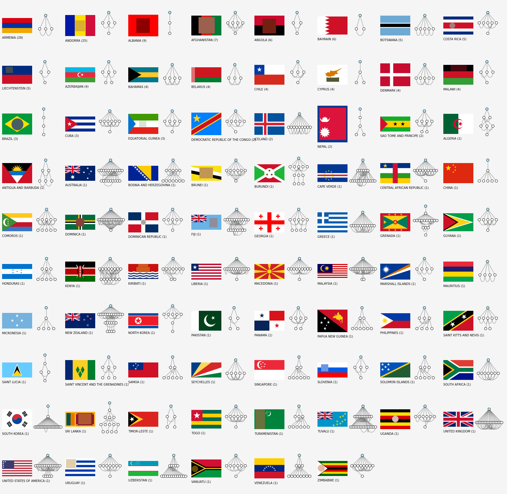
There are, in total, 78 classes. It turns out that quite a few countries display starts in their flags the number of which varies greatly. This is the main contributing factor to this large number of classes.
The non-singleton classes with their cardinalities are plotted below.
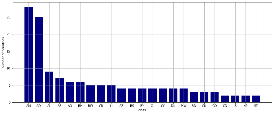
Each class is identified by the label of the country whose country code happens to come first alphabetically. For example,
- tricolor flags created by parallel splits: AM: Armenia
- bicolor flags with a coat of arms touching both rectangles: BH: Bahrein
- single field with a coat of arms of an other object on it: AL: Albania
In general, the more nodes and edges a flag has the fewer of its like can be found.
Inheritance
One can quickly recognise the some flags can be derived from other via simple manipulations
- splitting or encircling a region
- merging regions
For instance,
- take the Albanian flag
- encircle a region outside of the crest: the Cyprus class is created
- encircle a region inside of the crest: the Brazil class is created
- split the base rectangle on each side of the crest: The Angolan class is created
- split the base avoiding the crest: the Liechtenstein class is created
or
- take the flag of Bahrain
- split one of its fields so the new one only connects to the original field: the Armenian class is created.
- split one of its fields so the new one connects to both of the original fields: the Belarus class is created
By the repeated application of splits and merges all flags can be created from a few simple ones. These operations correspond to adding (or removing) nodes and edges. In graph parlance, if a subgraph of a graph is isomrophic to a full graph, it can be derived from the smaller graph. Therefore finding subgraph isomorphisms is equivalent to determining the family tree of flags in oru case.
Implementation
A graph from each class is retreived:
class_graphs = [x for x in graphs if x[0] in classes.keys()]
A directed graph is built. Each node of it is a flag graph. An edge point from a parent to its child. If $\mathcal{G}$ is a subgraph of $H$ then $G$ is a parent of $H$ and an edge $(G, H)$ is added to the family graph.
The edges are located by the GraphMatcher:
edges = []
for i, (k1, g1) in enumerate(class_graphs):
    for k2, g2 in class_graphs[i+1:]:

        if len(g1) > len(g2):

            matcher = GraphMatcher(g1, g2, node_match=match_node_type_single)
            is_subgraph = matcher.subgraph_is_isomorphic()

            if is_subgraph:
                edges.append((k2, k1))

        elif len(g1) < len(g2):

            matcher = GraphMatcher(g2, g1, node_match=match_node_type_single)
            is_subgraph = matcher.subgraph_is_isomorphic()

            if is_subgraph:
                edges.append((k1, k2))

        # isomorphism -- already handled
        else:
            continue
The family tree is created from the edges.
family_tree = nx.DiGraph()
family_tree.add_edges_from(edges)
The resultant tree, however, contains not only the immediate parent–child, but the greatparent–child and higher level connections. These are removed to have a clean tree. get_clean_levels works is two steps. Firstly, all offsprings of each generation are found starting from the head. The second step removes those descendants who are not immediately linked to any of their ancestors.
def get_clean_levels(g):
    # find top level
    heads =[x[0] for x in g.in_degree() if x[1] == 0]

    # find all children
    parents = set(heads)
    successors = []
    for i in range(len(g)):
        children = set(chain(*(g.successors(p) for p in parents)))
        if len(children) == 0:
            break
        successors.append(children)
        parents = children

    # remove non-immediate children
    clean = [set(heads)]
    for i, level in enumerate(successors):
        clean.append(level - set(chain(*successors[i+1:])))

    return clean
The create_clean_graph utility constructs a graph from these one egde long connections.
def create_clean_graph(g, levels):
    h = nx.DiGraph()
    for l1, l2 in zip(levels[:-1], levels[1:]):
        edges = (e for e in product(l1, l2) if e in g.edges)
        h.add_edges_from(edges)

    return h
The two functions applied in sequence yield a clean family tree.
levels = get_clean_levels(family_tree)
family_tree_clean = create_clean_graph(family_tree, levels)
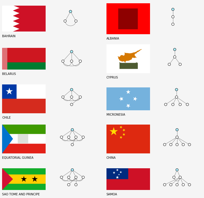
The family tree of all classes are displayed below. There are two head nodes Bahrain and Albania. Both have two nodes (or regions). They cannot be derived from each other by adding nodes. All of the flags can be constructed from these two by splitting regions or adding new ones.
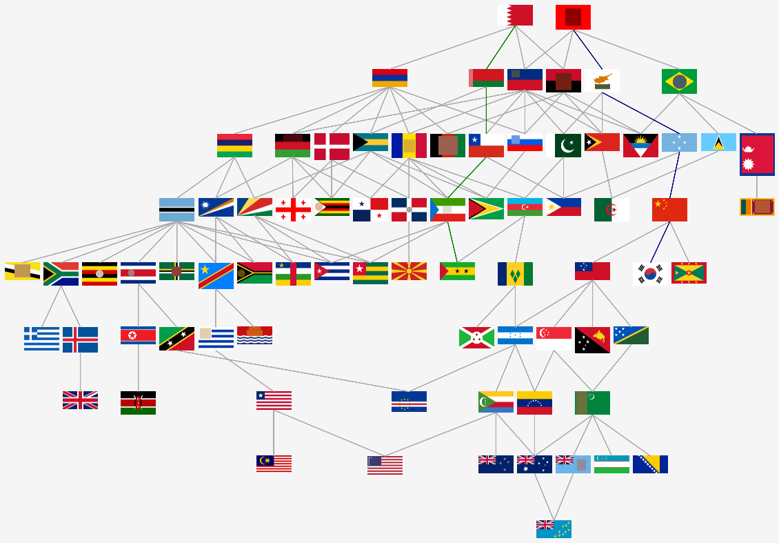
Two paths are examined in detail.
Bahrain to Sao Tome and Principe (green trail)
- A new segment is attached to the flag of Bahrain that touches both of the original segments and the border. This yields the class of Belarus. The new segment is the node in the middle node.
- An enclave is created inside of the latest segment generating the class of Chile. The new node is placed in the third tier on its own.
- The green (or equivalently, the red) rectangle is adde to the flag which generates the Equatorial Guinea class. The new node is the one on the right n the middle tier.
- A star is added (circular split) to obtain the Sao Tome and Principe class. The corresponding node is one in the third tier.
Albania to Samoa (blue trail)
- An other enclave is created adding a second child node in the third tier forming the Cyprus class.
- Two more stars are split out from the canvas increasing the number of child nodes to four. The created class belongs to Micronesia.
- Yet an other star is added to get the China class. The number of child nodes are now five.
- Attaching a region to the Chinese flag creates the Samoa class. The node corresponing to the latest region is in the second tier, without any children.
