Markov cluster algorithm

Motivation

Graph clusters

When looking at certain graphs, one immediately recognises that certain nodes are grouped together. This perceived grouping can base on the number of edges between the nodes in question, or on some other quality that links the nodes; e.g. a similarity measure. Either way, edges represent a weight which is generally larger between nodes in a group than between those inside and outside of the group. We would like to identify these group. The process to achieve this is called graph clustering.

Markov process

Imagine that there is person standing on a node of the graph. He can only step to nodes which are link to the one he rests on. Once he is on the new he can move an other one no matter where he stood before. This is an example of the Markov process where the transition from one state to the other does not depend on the previous states leading to the current one. If this random walker happens to be in a region where the nodes are strongly connected, he is likely to spend more time there. In other words connected nodes that have high step count are clusters in this sense.

The Markoc Cluster algorithm is based on this analogy, which are going to implement. The source code can be found here.

Formulation

Transition probabilities

Let us denote each node with an integer in a graph. The probability of going from node $i$ to node $j$ is the weight of the edge leading from $i$ to $j$ divided by the sum of weights originating from node $i$:

The transition matrix thus can be expressed as the row normalised adjacency matrix.

A few remarks are in order:

1. Our graph is digraph with at most two parallel edges
2. There are no loops in the graph
3. In most of the literature on MC the transition matrix is the column normalised adjacency matrix. It is arbitrary to make this choice provided the normalisation is applied consistently throughout the process. I chose row normalising because the sparse matrix operations are implemented in compressed row format in python.

Repeated random steps

In general, the probability of going from $i$ to $j$ is proportional of the product of the corresponding row and column

which is just the matrix product. This step is called expansion intuitively enough.

What do we expect?

1. Larger backflow between nodes that are strongly connected.
2. Central nodes will have larger probabilities to arrive at

If we multiply the matrix enough times we get the stationary distributions as the rows..

What we really want to do is to gradually remove those edges which represent small transition probabilities and reassigning these probabilities to the larger ones. This can be achieved by forming the Hadamard (elementwise) product of the matrix and renormalising the rows. (Elementwise exponentiation has the same effect as multiplication provided the exponent is larger than one.) This step is called inflation.

If we keep expanding and inflating the transition matrix we will have only a selection of central nodes with large incoming probabilities. These groups of nodes are the clusters. It will have either zero columns or columns that are equal but not zero. It is easy to prove that such a matrix is doubly idempotent that is its square equals to itself.

Algorithm

The Markov cluster algorithm can be summarised as follows:

The $\texttt{Inflate}$, $\texttt{Expand}$ functions inflate and expand the transition matrix as defined in the previous paragraph. $\texttt{Prune}$ removes all elements below a threshold. $\texttt{RowNormalise}$ normalises each row to unit in $L1$ sense. Finally, $\texttt{ReadClusters}$ compares the column vectors to assign cluster labels to the nodes (see my previous post).

Implementation

I have implemented the Markov cluster algorithm both purely in numpy and using scipy.sparse. The repos can be found here.

Implementation considerations

The main concern was to create an efficient implementation. The following observations guided me:

1. Many elements are zero in the transition matrix $\rightarrow$ use sparse matrix
2. Large volume of data $\rightarrow$ try to use inplace operations
3. Many elements become zero $\rightarrow$ update (prune) matrix repeatedly
4. Be similar to sklearn utilities $\rightarrow$ implement as a class
5. Be flexible for future development $\rightarrow$ see above

Example

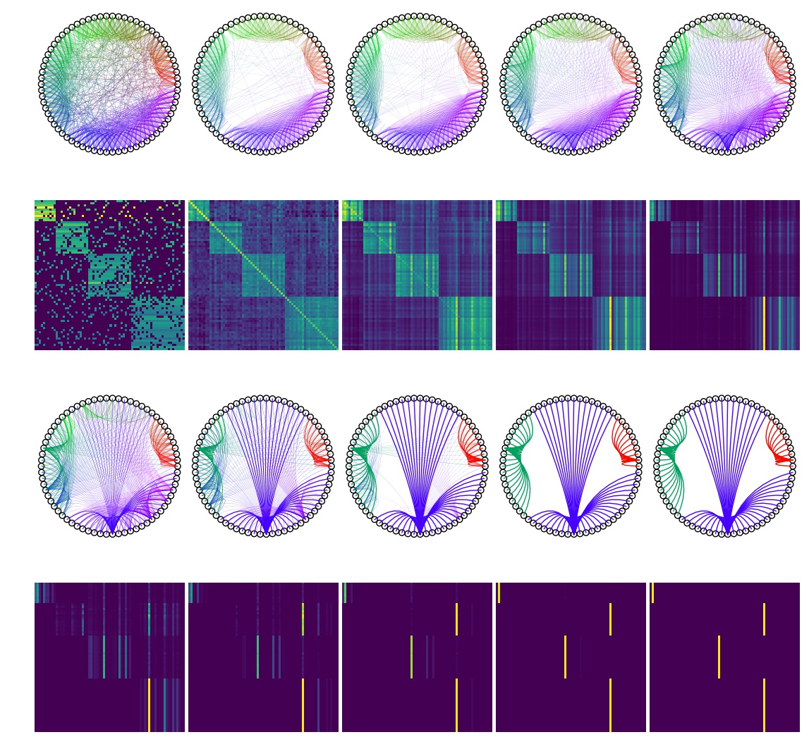
The Markov cluster algorithm is best illustrated in small datasets (it is also beneficial if we do not intend to wait for plotting the graphs with pyplot until doomsday). For this end a graph with hundred nodes is generated. The graph consist of four almost complete subgraph that are linked to each other.

import networkx as nx
random_graph = nx.random_partition_graph([10,15,20,25], 0.8, 0.15, seed = 41)
adj_mat = nx.adjacency_matrix(random_graph)

We can now invoke the MC algorithm:

import sys
sys.path.append(r'C:\Users\Balazs\source\repos\MPC\MPC\MCSparse')
from MCSparse import MCsparse

mclus = MCsparse(diag_scale = 1.0, expand_power = 2, inflate_power = 2.0,
                    max_iter = 30, save_steps = 2, threshold = 1.0e-6, tol = 1.0e-17)

mclus.fit(adj_mat)

Iteration 0 : diff 68.62072426791217
Iteration 1 : diff 24.576930893277975
Iteration 2 : diff 20.13319519548316
Iteration 3 : diff 16.248431243559647
Iteration 4 : diff 13.053582190304283
Iteration 5 : diff 7.580491155035162
Iteration 6 : diff 1.2659174615866695
Iteration 7 : diff 0.12656809852558704
Iteration 8 : diff 0.001710578902421697
Iteration 9 : diff 0.0


C:\Users\Balazs\Anaconda3\lib\site-packages\scipy\sparse\compressed.py:730: SparseEfficiencyWarning: Changing the sparsity structure of a csr_matrix is expensive. lil_matrix is more efficient.
  SparseEfficiencyWarning)





<MCSparse.MCsparse at 0x1492adaf4e0>

The warning only notifies us that the diagonal has been changed. We can safely ignore it. As we can see, the matrix becomes idempotent in nine iterations. The transition matrix and the clusters are shown below for each iteration. The cluster labels are accessed as:

print(mclus.labels_)

[0 0 0 0 0 0 0 0 0 0 2 2 2 2 2 2 2 2 2 2 2 2 2 2 2 1 1 1 1 1 1 1 1 1 1 1 1 1 1 1 1 1 1 1 1 2 2 2 2 2 2 2 2 2 2 2 2 2 2 2 2 2 2 2 2 2 2 2 2 2]

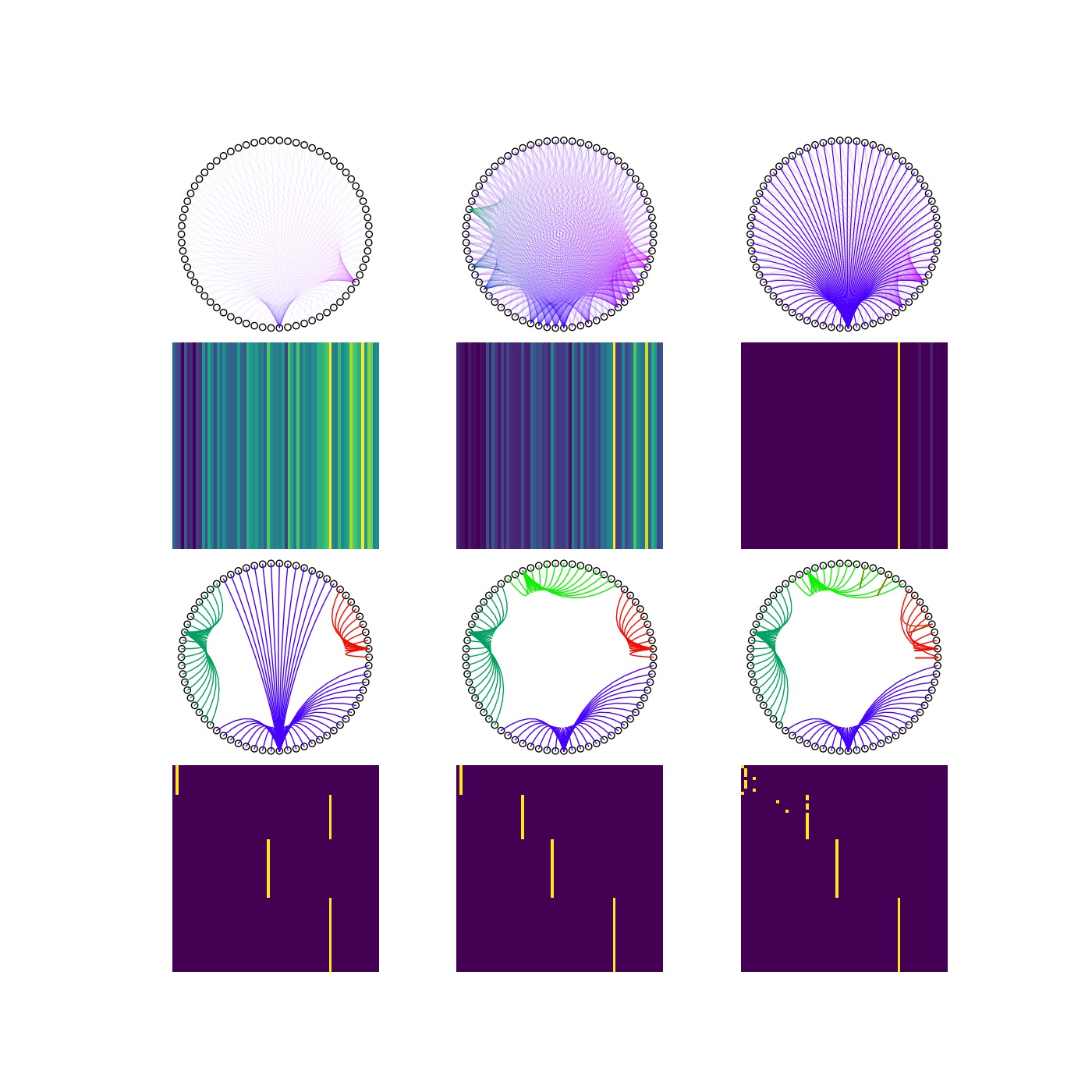
Changing the inflation parameter changes the cluster structure. The lower the inflation parameter, that is the rate of removal of edges with lower weights the larger clusters we get.

This effect on the final cluster sizes is illustrated on a larger set of inflation parameters: $q=[1.00, 1.20, 1.50, 2.00, 2.25, 3.00]$, below.

Analysis

Most of the clustering methods minimise a ceratian measure (e.g. variance of the intra-cluster distance in k-means clustering). However, it is not clear from above what functional of the graph is minimised during the MC algorithm. It is also curious that changing the rate of inflation changes the cluster structure.

Nevertheless, one can show that the entropy is the Markov process, $S(\mathbf{P})$, is minimised.

where $\mathbf{\mu}$ is the left eigenvector of the stochastic matrix.

The function calc_markov_entropy calculates the entropy of the transition matrix relative to the entropy of the process where each state has equal probability to move to any other states. The entropy is the corresponding process is $\log_{2}(n)$.

def calc_markov_entropy(mat):
    """
    Calculates the entropy of the Markov process.
     Parameters:
        mat (scipy.sparse.csr_matrix) : transition (stochastic) matrix
    Returns:
        entropy (float) : relative entropy wrt fully connected Markov process.
    """
    v, vec = sps.linalg.eigs(mat.transpose(), k = 1)
    vec = vec / vec.sum()

    mat.data = mat.data * np.log2(mat.data) 
    entropy = - np.sum(np.multiply(mat.sum(axis = 1), np.real(vec))) / np.log2(mat.shape[0])
        
    return entropy

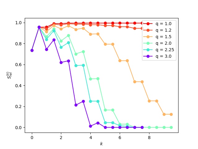
The entropies have been calculated for each inflation (even) and expansion (odd) steps for each of the above inflation parameters.

It is readily observed that the entropy increases during the expansion set and decreases following inflation. These changes gradually diminish as the matrix becomes idempotent.

I will write about the properties of the Markov cluster algorithm in an other post. For now, it suffices to note,

1. MC reminds us of the expectation maximisation algorithms. The expectation step is the expansion the maximisation step is the inflation.

1. It also alludes to the simulated annealing algorithm. Expansion corresponds to increasing the energy of the system, whereas the inflation parameter has a similar role to that of the cooling rate. 

1. Depending on the inflation parameter one can build a hierarchy of cluster.