Itinerary
We are going to explore the structure of domestic flight routes in a number of countries. This will involve the following steps:
- Gathering data from public databases
- Cleaning and restructuring the data
- Analysing the data by means of clustering
- Attempting to say clever things
- Visualising the data
Motivation
I am fascinated by airports and, in general, by flying. I hope this is a sufficient reason.
Before setting off
Choosing the first destination
First of all, it has to be decided what will be investigated. We are going to look at the domestic routes in a selection of countries. The next question is whether individual networks are investigated, or beyond that, we carry out a comparative study across countries. Initially, we only concern ourselves with countries apiece.
Secondly, it has to be decided whether certain features are sought for, or the structure of the routes is let gradually unfold? As a start we will look for clusters in the route network.
Finding the right guidebook
It is of considerable challenge to decide whether the number of cluster measures exceeds that of the clustering algorithms.
Let us consider a simple graph $G = (V,E)\text{ where } E \in V^{2}$ whose edges are partition non overlapping non empty sets: $V = \cup_{i = 1}^{N} C_{i}$. The graph induced by such a set is called a cluster.
As to decide what constitutes a good cluster, two requirements are cited most often:
- The number of edges within a cluster is much higher than that of edges linking the cluster in question to other ones.
- The edge density e.g. the average degree of vertices with respect to the edges within the cluster is high.
Bearing these in mind, we can attempt to construct a measure. Firstly, the “trapping probability”, $p_{trap}(i)$ for a vertex as the probability of moving to a neighboring vertex within the cluster over the probability to move any neighboring vertex. Assuming that the vertex $i$ belongs to cluster $k$:
\[p_{tr}(i) = \begin{cases} 1, \quad \quad \quad \quad\text{if} \quad |E(C_{k})| = 0\\ \frac{ \sum\limits_{(i,j) \in E(C_{k}) } w((i,j)) } {\sum\limits_{(i,j)} w((i,j))} , \quad \text{if} \quad |E(C_{k})| > 0\\ \\ \end{cases}\]where $w(i,j)$ is the weight of the edge between vertices $i$ and $j$. All edges are required to have non-negative weight. Self edges are not allowed either. This quality is bounded between 0 and 1.
The cluster trapping probability, $p_{tr}(C_{k})$ is the average of the trapping probabilities over its vertices:
\[p_{tr}(C_{k}) = \frac{\sum\limits_{i \in C_{k}} p_{tr}(i) } {|C_{k}|}\]Obviously, this the values of this quality are confined between 0 and 1. The former meaning a cluster with a single vertex connected to other clusters, whilst the latter one singifies a cluster disjoint from any other clusters.
Based on this measure one can devise a clustering algorithm where vertices are sequentially added or removed whether they increase of decrease the trapping probability. However, this measure is biased towards large clusters for the trapping probability of any cluster that is composed of a connectedted standalone graph is unity.
Therefore we consider the second criterion that requires high intra cluster edge density. Naively, one can define the desity as the sum of the intra cluster edges over the maximum possible number of intra cluster edges:
\[g(C_{k}) = \frac{ |E(C_{k})|}{ {|C_{k}| \choose 2} }\]However, if the edges have non-uniform weights the expression above is not bounded between 0 and 1 anymore. To rectify this, the weights are normalised by the maximum weight in the entire graph, $w_{max}$.
\[\tilde{w}(ij) = \frac{w(ij)}{w_{max}}\] \[p_{sat}(C_{k}) = \frac{\sum\limits_{(ij) \in E(C_{k})} \tilde{w}(ij)} { {|C_{k}| \choose 2} }\]This measure works the best if the variance of the weights is small and there are no outliers towards large values. In that case one can further scale the weights with the probability distribution function of them.
Finally the two measures can be combined into one:
\[m(C_{k}) = \alpha p_{tr}(C_{k}) + (1 - \alpha) p_{sat}(C_{k}) \, , \quad \alpha \in [0,1]\]The cluster quality of the whole graph is the average of the individual cluster measures:
\[m(G) = \frac{\sum\limits_{C_{k} \in C} m(C_{k})}{|C|}\]A scipy.sparse implementation is found below.
import numpy as np

def calculate_c_score(X, labels, alpha = 0.50):
    """

    """

    # separate labels into clusters
    clusters = {label : np.argwhere(labels == label).flatten() for label in np.unique(labels)}

    nc = len(clusters) # number of clusters
    w_max = X.max()    # maximum weight

    p_trap = 0         # trapping probability
    p_sat = 0          # edge density

    for label, idcs in clusters.items():
        nv = idcs.size

        if nv == 1:
            p_trap += 1.0; p_sat += 1.0

        else:
            # sum of weights in cluster
            w_intra_sum = X[idcs[:,None], idcs].sum(axis = 1)

            # sum of weights going out of cluster
            w_extra_sum = X[idcs].sum(axis = 1)  - w_intra_sum

            # trapping probability
            p_trap += np.mean(w_intra_sum / (w_intra_sum + w_extra_sum))

            # saturation
            p_sat += np.sum(w_intra_sum) / (nv * (nv - 1) / 2 * w_max)

    p_trap /= nc; p_sat /= nc;
    c_score = alpha * p_trap + (1.0 - alpha) * p_sat

    return (c_score, p_trap, p_sat, alpha)
Choosing the right guide
Choosing the algorithms with which the data are transformed is strongly related to the question above. We will use Markov cluster algorithm and hierarchical clustering to find clusters. The latter one cab also be used to uncover the generic structure of the graphs.
Gathering the data
I wrote a scraper (‘lxml.html’ with ‘xpath’ expressions) that pulls the all routes from the appropriate Wikipedia pages. (It was as delightful to write it as it sounds, thus I save the reader from the details). The raw data are stored in json format.
It contains the
- the name of the airport as index
- A dictionary of airlines serving that airport and their destinations
{airline1 : [dest11, dest12, ...], airline2 : [dest21, dest22, ...], ...} - the aliases i.e. alternative names of the airport
- the geographical coordinates
- the IATA code
- the name
The first two lines of the Japanese network database look like:
import pandas as pd

path_to_airport_file = r'C:\Users\Balazs\source\repos\AirportScraper\AirportScraper\airports_by_country\JPN_airport_connectivity.json'
df = pd.read_json(path_to_airport_file, orient = 'index')
df.head(5)
| AIRLINES_DEST | ALIASES | COORDS | IATA | NAME | |
|---|---|---|---|---|---|
| AGUNI_AIRPORT | {'/wiki/First_Flying': ['NAHA_AIRPORT']} | [AGUNI_AIRPORT, AGUNI_(AIRPORT)] | [26.59278, 127.24028] | AGJ | AGUNI_AIRPORT |
| AKITA_AIRPORT | {'/wiki/All_Nippon_Airways': ['CHUBU_CENTRAIR_... | [AKITA_AIRPORT, AXT, RJSK] | [39.61556, 140.21861] | AXT | AKITA_AIRPORT |
| AMAMI_AIRPORT | {'/wiki/Japan_Airlines': ['KAGOSHIMA_AIRPORT',... | [AMAMI_AIRPORT, AMAMI_(AIRPORT), AMAMI_O_SHIMA... | [28.43083, 129.71250] | ASJ | AMAMI_AIRPORT |
| AOMORI_AIRPORT | {'/wiki/All_Nippon_Airways': ['ITAMI_AIRPORT',... | [AOMORI_AIRPORT] | [40.73333, 140.68861] | AOJ | AOMORI_AIRPORT |
| ASAHIKAWA_AIRPORT | {'/wiki/Air_Do': ['HANEDA_AIRPORT'], '/wiki/Al... | [ASAHIKAWA_AIRPORT, RJEC] | [43.67083, 142.44750] | AKJ | ASAHIKAWA_AIRPORT |
Preparing the data
The “ARILINES_DEST” column still contains the international routes which have to be removed. The coordinates have to be converted to floats too. We will need a few standard library functions.
from collections import Counter
from itertools import chain
Firstly, we move the index to a column
df.reset_index(inplace = True)
df['AIRPORT_NAMES'] = df['index']
The coordinates are then converted to floats
df['COORDS'] = df['COORDS'].apply(lambda x: list(map(lambda y: float(y), x)))
The number of airlines serving an airport:
df['NUM_AIRLINES'] = df['AIRLINES_DEST'].apply(lambda x : len(x))
Number of destinations (not checked for duplicates) is the sum of the length of the destination lists:
df['NUM_DESTINATIONS'] = df['AIRLINES_DEST'].apply(lambda x : sum(map(lambda _x : len(_x), x.values())))
The unique destinations can be found by creating the union of all destinations, from which the number of them can easily be found:
df['UNIQUE_DESTINATIONS'] = df['AIRLINES_DEST'].apply(lambda x : list(set(chain(*x.values()))))
df['NUM_UNIQUE_DEST'] = df['UNIQUE_DESTINATIONS'].apply(lambda x : len(x))
To find the domestic routes a list of domestic ariports is created
sel = df['AIRPORT_NAMES'].values
Below, x is a dictionary {airline1 : [dest11,..], airline2 : [dest21, ...]} from which we select those destinations which are in sel. Then we reconstruct the dictionaries using these destinations.
df['INTERNAL_DEST'] = \
df['AIRLINES_DEST'].apply(lambda x : {_key : list(filter(lambda _v : _v in sel, _val)) for _key, _val in x.items()})
Those airlines which have zero domestic destinations are then removed:
df['INTERNAL_DEST'] = df['INTERNAL_DEST'].apply(lambda x : dict(filter(lambda x : len(x[1]) > 0, x.items())))
For each airport we create a summary of destinations:
df['INTERNAL_ROUTES'] = df['INTERNAL_DEST'].apply(lambda x : Counter(chain(*x.values())))
As a final step, the airport names are replaced by their respective indices. The field ‘INTERNAL_ROUTES’ is a dictionary where the keys are the airport indices whereas the values are the number of routes.
df['INTERNAL_ROUTES'] = \
df['INTERNAL_ROUTES'].apply(lambda x : {df.index[df['AIRPORT_NAMES'] == _key].tolist()[0] : _val for _key, _val in x.items()})
If we are only interested in the internal routes they can be transfered to a different dataframe along with other useful attributes.
keep_columns = ['COORDS', 'IATA', 'NAME', 'INTERNAL_ROUTES']
df_clean = df.filter(keep_columns, axis=1)
df_clean.head(5)
| COORDS | IATA | NAME | INTERNAL_ROUTES | |
|---|---|---|---|---|
| 0 | [26.59278, 127.24028] | AGJ | AGUNI_AIRPORT | {42: 1} |
| 1 | [39.61556, 140.21861] | AXT | AKITA_AIRPORT | {6: 1, 17: 2, 45: 2, 13: 1} |
| 2 | [28.43083, 129.7125] | ASJ | AMAMI_AIRPORT | {22: 1, 24: 1, 54: 1, 66: 1, 76: 1, 42: 1, 23:... |
| 3 | [40.73333, 140.68861] | AOJ | AOMORI_AIRPORT | {17: 2, 45: 2} |
| 4 | [43.67083, 142.4475] | AKJ | ASAHIKAWA_AIRPORT | {13: 2, 6: 1, 23: 1, 17: 1} |
The journey
Dataframes are useful one wishes to store and manipulate the data in a convenient way. However, graps provided by networkx seem a more natural data format.
A graph of the domestic routes called routes can then be created from the condensed adjacency list in column INTERNAL_ROUTES.
import networkx as nx

def df_to_nxgraph(df, edge_name, keep_node_attributes = {}):
    """
    Creates an networkx graph representation of of the airport routes.
    Parameters:
        df (pd.Dataframe) : dataframe object of the airports
        edge_name (str) : name of the column which contains the routes as a dictionary
    Returns:
        routes (nx.Graph) : undirected graph with airport indices as nodes.
    """
# create a list of edges
    adjacency_list = dict(zip(df.index.values, df[edge_name].values))
    adjacency_list = [(source, target, weight) for source, destination in adjacency_list.items()
                                                   for target, weight in destination.items()]

# initialise graph
    route_graph = nx.Graph()
    route_graph.add_nodes_from(df.index.values.tolist())
    route_graph.add_weighted_edges_from(adjacency_list)

# save selection of attributes
    for node_attr_name, col_name in keep_node_attributes.items():
        attribs = dict(zip(df.index.values, df[col_name].values))
        nx.set_node_attributes(route_graph, attribs, node_attr_name)

    return route_graph
route_graph = df_to_nxgraph(df_clean, 'INTERNAL_ROUTES',
                            keep_node_attributes = {'COORDS' : 'COORDS'})

adjmat = nx.adjacency_matrix(route_graph)
There is an other reason to use graphs: the network is sparse, so that storing and manipulating only the existing edges improves the performance.
n_nodes = route_graph.number_of_nodes()
sparsity = route_graph.number_of_edges() / (n_nodes * (n_nodes - 1)) * 100
print("Sparsity: {0:4.2f}%".format(sparsity))
Sparsity: 3.98%
Clustering
Firstly, we use our Markov cluster algorithm.
import sys
sys.path.append(r'C:\Users\Balazs\source\repos\MCA\MCA\MCAsparse')
sys.path.append(r'C:\Users\Balazs\source\repos\MCA\MCA')
from MCAsparse import MCsparse
from matplotlib import pyplot as plt

# create adjacency matrix
adjmat = nx.to_scipy_sparse_matrix(route_graph, weight = 'weight')
adjmat = (adjmat + adjmat.T) / 2.0

# initialise classifier
mclus = MCsparse(diag_scale = 1.0, expand_power = 2, inflate_power = 2.0,
                 max_iter = 30, save_steps = 1, threshold = 1.0e-5, tol = 1.0e-17)

# perform clustering and get labels
labels = mclus.fit_predict(adjmat)

print("\nNumber of clusters: {0}\n".format(np.unique(labels).size))
print("labels: ", labels)
Iteration 0 : diff 87.57589200951395
Iteration 1 : diff 36.27147570473598
Iteration 2 : diff 23.983993398453297
Iteration 3 : diff 6.911031173875251
Iteration 4 : diff 1.1179346870855424
Iteration 5 : diff 0.10509041232629668
Iteration 6 : diff 0.0022368650642770223
Iteration 7 : diff 0.0

Number of clusters: 4

labels:  [2 3 3 3 3 0 1 1 3 3 1 3 3 1 3 3 1 1 1 3 3 0 3 3 3 2 3 3 3 3 2 3 3 3 3 1 2
 1 0 2 3 3 2 3 3 3 2 3 3 0 1 3 1 3 3 1 3 0 3 3 3 3 1 3 2 3 3 3 1 3 1 3 3 3
 1 2 3]


C:\Users\Balazs\Anaconda3\lib\site-packages\scipy\sparse\compressed.py:730: SparseEfficiencyWarning: Changing the sparsity structure of a csr_matrix is expensive. lil_matrix is more efficient.
  SparseEfficiencyWarning)
Sights to see
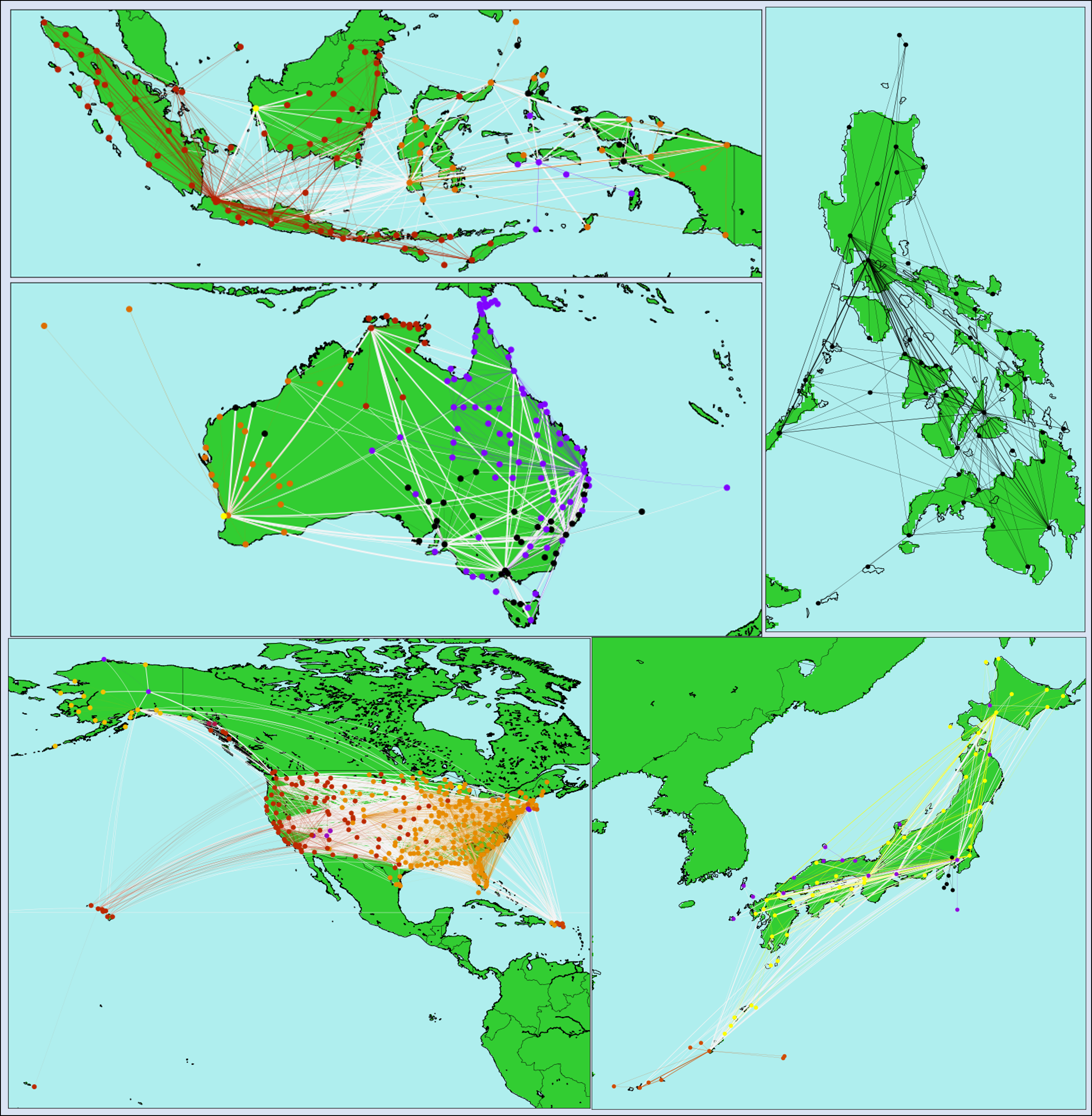
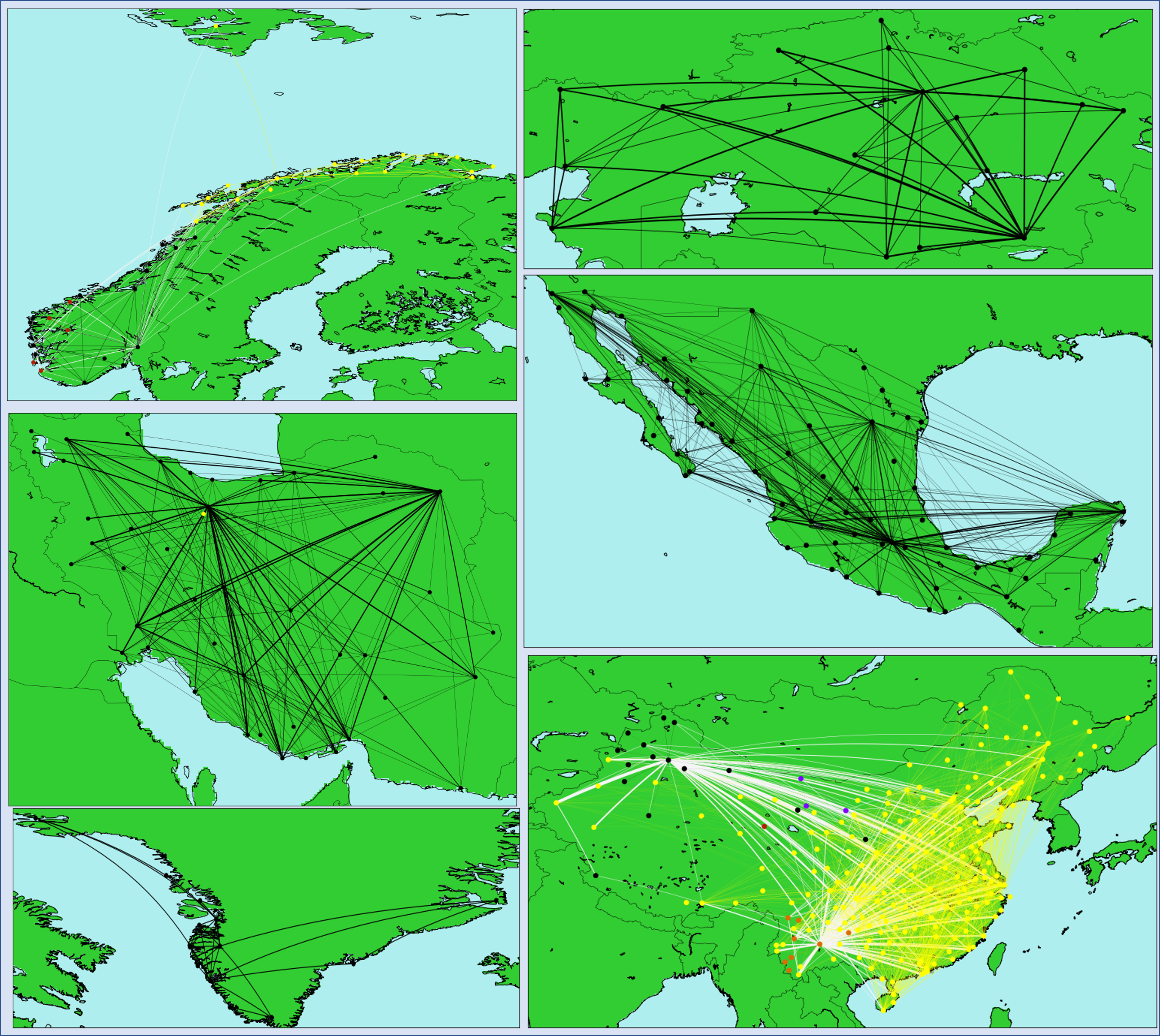
A number of domestic networks are shown below. (The countries are not labeled on purpose, it is expected that the kind reader recognises them.) The intra cluster routes are coloured according to the cluster they belong. The inter cluster routes are in lightgrey colour.


A few remarks are in order.
- If there are more than one clusters, the members of each cluster tend to be close to each other in geographical sense.
- There is also a few examples where a set of destinations are only available from a certain airport (see Japan).
- Local routes between groups of islands are separated (see Japan again).
- There are singleton clusters: These are airports with none (i.g. Imam Khomeini in Tehran) or very few domestic routes.
- In order to unravel the relationship between the Markov clusters and geography of the network one can perform a clustering based on geographycal distances. The two groupings can then be compared.
- There are a few clusters where some members are not connected to the main body of the cluster by intra cluster routes. Nevertheless, it is more likely to travel to the other members of the cluster by means of random walk.
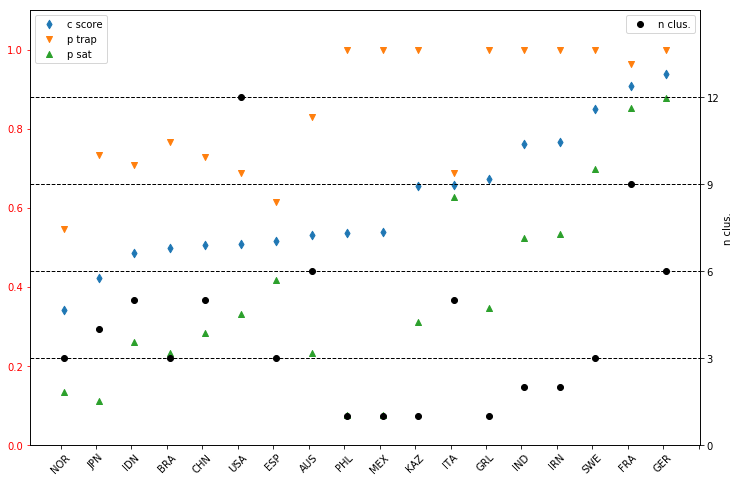
The composite score has been calculated for all countries which are shown below. It is delightful to see that the edge density (green upward triangles) is low when there is only one cluster. (Please remember, this measure was not minimised explicitly during the classification.)

The trapping probability, in general, is high. This is due to the fact that each cluster contributes equally to $p_{trap}$. It can be made more balanced the averaged is weighted with the size of the cluster. Nevertheless, it is unit when there is only one cluster, as it is expected to be.
Trip report
We have analysed the domestic air routes for a number of countries using Markov cluster algorithm. Geographical segmentation of the networks has been observed. However, the current algorithm resulted one cluster in many cases, hiding the internal structure of the routes.
Future journeys
We will try to use agglomerative clustering to build a hierarchy of the flight networks.